Visualization, Quantification, and Mapping of Immune Cell Populations in the Tumor Microenvironment

Summary

Here, we describe a simple and accessible strategy for visualizing, quantifying, and mapping immune cells in formalin-fixed paraffin-embedded tumor tissue sections. This methodology combines existing imaging and digital analysis techniques with the purpose of expanding the multiplexing capability and multiparameter analysis of imaging assays.

Abstract

The immune landscape of the tumor microenvironment (TME) is a determining factor in cancer progression and response to therapy. Specifically, the density and the location of immune cells in the TME have important diagnostic and prognostic values. Multiomic profiling of the TME has exponentially increased our understanding of the numerous cellular and molecular networks regulating tumor initiation and progression. However, these techniques do not provide information about the spatial organization of cells or cell-cell interactions. Affordable, accessible, and easy to execute multiplexing techniques that allow spatial resolution of immune cells in tissue sections are needed to complement single cell-based high-throughput technologies. Here, we describe a strategy that integrates serial imaging, sequential labeling, and image alignment to generate virtual multiparameter slides of whole tissue sections. Virtual slides are subsequently analyzed in an automated fashion using user-defined protocols that enable identification, quantification, and mapping of cell populations of interest. The image analysis is done, in this case using the analysis modules Tissuealign, Author, and HISTOmap. We present an example where we applied this strategy successfully to one clinical specimen, maximizing the information that can be obtained from limited tissue samples and providing an unbiased view of the TME in the entire tissue section.

Introduction

Cancer development is the result of a multistep process involving reciprocal interactions between malignant cells and the TME. Other than tumor cells, the TME is composed of nonmalignant cells, stromal cells, immune cell populations, and extracellular matrix (ECM)¹. The spatial organization of the different cellular and structural components of the tumor tissue and the dynamic exchange between the cancer and neighboring non-cancer cells ultimately modulate tumor progression and response to therapy^2,3,4. It has been shown that the immune response in cancer is spatiotemporally regulated^5,6. Different immune cell populations infiltrating the neoplastic lesion and the adjacent tissue exhibit distinctive spatial distribution patterns and varied activation and differentiation states associated with different functions (e.g., pro- versus antitumor). These different immune populations and their parameters coevolve overtime with the tumor and the stromal compartments.

The emergence of technologies allowing single cell multiomics profiling has exponentially increased our understanding of the numerous cellular and molecular networks regulating carcinogenesis and tumor progression. However, most single cell-based high-throughput analytical tools require tissue disruption and single cell isolation, resulting in loss of information about the spatial organization of cells and cell-cell interactions⁷. Because the location and arrangement of specific immune cells in the TME have diagnostic and prognostic value, technologies allowing spatial resolution are an essential complement of single cell-based immune profiling techniques.

Traditionally, imaging techniques like immunohistochemistry (IHC) and multiplex immunofluorescence (mIF) have been restricted to a small number of biomarkers that can be visualized simultaneously. This limitation has hampered the study of the spatiotemporal dynamics of tumor-infiltrating immune cells, which are typically defined by several phenotypic markers. Recent advances in imaging and analytical tools have expanded the possibilities of multiplexing. New antibody-based labeling technologies like histo-cytometry and imaging mass cytometry have been used to spatially separate up to 12 and 32 biomarkers, respectively^8,9. Mass spectrometry imaging, a technique not requiring labeling, has the potential to image thousands of biomarkers simultaneously in a single tissue section^10,11. Although these techniques have already shown great potential for dissecting the tissue immune landscape in cancer, they use highly sophisticated and expensive equipment and software and are not readily accessible to the majority of researchers.

Alternatively, the multiplexing capability of traditional IHC and mIF has been expanded through the use of serial imaging, sequential rounds of labeling, and spectral imaging^{7,12,13,14,15,16}. These techniques generate multiple images from the same or from serial tissue sections that can be consolidated into virtual multiparameter slides using image analysis software. As a result, the number of markers that can be visualized and analyzed simultaneously increases.

Here, we propose a strategy for the rational design of tissue multiplex assays using commercially available reagents, affordable microscopy equipment, and user-friendly software (Figure 1). This methodology integrates serial imaging, sequential multiplex labeling, whole tissue imaging, and tissue alignment to generate virtual multiparameter slides that can be used for automated quantification and mapping of immune cells in tissue sections. Using this strategy, we created one virtual slide comprising 11 biomarkers plus two frequently used histological stains: hematoxylin and eosin (H&E) and picrosirius red (PSR). Multiple immune cell populations were identified, located, and quantified in different tissue compartments and their spatial distribution resolved using tissue heatmaps. This strategy maximizes the information that can be gained from limited clinical specimens and is applicable to formalin-fixed paraffin-embedded (FFPE) archived tissue samples, including whole tissue, core needle biopsies, and tissue microarrays. We propose this methodology as a useful guide for designing custom assays for identification, quantification, and mapping of immune cell populations in the TME.

Protocol

Three serial FFPE sections from resected hepatitis B virus (HBV)-associated human hepatocellular carcinoma were obtained from the Centre hospitalier de l'Université de Montréal (CHUM) Hepatopancreatobiliary Cancer Clinical Database and Biological Specimen Repository (HBP Biobank). Patients participating in this tissue bank provided informed consent. This study was approved by the institutional ethics committee (Protocol number 09.237) and performed in accordance with the Declaration of Helsinki.

1. Hematoxylin and eosin (H&E) staining protocol

NOTE: The H&E staining was performed by the molecular pathology core facility of the Centre de Recherches du Centre hospitalier de l'Université de Montréal (CRCHUM) using the Shandon multiprogram robotic slide stainer using the following program.

1. For deparaffinization, immerse slides 3x for 2.5 min each in xylene substitute.
   CAUTION: Xylene substitutes are flammable, skin irritants, and harmful if inhaled.
2. For rehydration, immerse slides in 100% ethanol 3x for 2.5 min each. Wash for 1 min in double distilled water (ddH₂O) to rehydrate.
3. Incubate for 1 min in hematoxylin. Wash 3x for 1 min each in ddH₂O.
4. Incubate for 5 s with eosin. Wash 30 s with 95% ethanol. Wash 2x for 1 min with 100% ethanol.
   CAUTION: Ethanol is flammable and an eye irritant. Eosin is an eye irritant.
5. For dehydration, immerse 3x for 1.5 min each in the xylene substitute. Mount slides manually.
   NOTE: The estimated time for executing this part of the protocol is 30 min.

2. Multiplex immunofluorescence staining protocol for FFPE sections

NOTE: This protocol was adapted from Robertson et al.¹⁷.

1. Deparaffinization and rehydration
   NOTE: Before antibody-mediated labeling of FFPE sections by IHC or mIF, the paraffin should be removed. Failure to efficiently remove the paraffin results in suboptimal staining.
   1. Place 4 μm FFPE tissue section slides into glass slide holders. Under the fume hood, immerse the slides in a Coplin jar containing 37°C prewarmed xylene for 10 min.
      CAUTION: Xylene is flammable, a skin irritant, and harmful if inhaled.
   2. Manually agitate the slides for 10 s every 2 min. Repeat 1x in fresh xylene for another 5 min.
   3. In the chemical hood, immerse the slides sequentially for 5 min in each of the following solutions: 1) xylene : ethanol (1:1 v/v); 2) 100% ethanol; 3) 70% ethanol; 4) 50% ethanol; 5) 30% ethanol; 6) phosphate-buffered saline (PBS).
      NOTE: Keep the slides in PBS until ready to perform the antigen retrieval. Keep the dewaxed sections hydrated at all times. Drying out will cause nonspecific antibody binding and therefore high background staining.
2. Heat-induced antigen retrieval
   NOTE: Antigens can be masked upon formalin-fixation, preventing antibody binding and consequently visualization. The use of antigen unmasking buffers and procedures partially reestablish the native conformation of epitopes and thereby restores antibody recognition. The type of antigen retrieval buffer and duration should be optimized for the specific assay conditions (e.g., target, antibody, tissue, etc.).
   1. Immerse dewaxed slides in a Coplin jar containing the antigen retrieval solution (recipe in Table of Materials).
   2. Place closed Coplin jar into an electric pressure cooker with tap water. The water level should not exceed half the height of the jar so that the water does not mix with the antigen retrieval solution.
   3. Close the lid and the pressure valve of the cooker. Select high pressure for 10 min and start. When done, unplug the cooker, release the pressure, open the lid, and keep the jar inside the cooker for 30 min, allowing the slides to cool.
3. Blocking of nonspecific binding
   1. Transfer the rack with the slides to a Coplin jar filled with PBS. Rinse off the antigen retrieval buffer with PBS 2x for 5 min each.
   2. Encircle the tissue sections with a PAP pen to create a hydrophobic barrier. Immerse the slides in a Coplin jar containing 0.1 M glycine in PBS. Incubate for 15 min at room temperature (RT).
      NOTE: Glycine saturates the aldehyde groups generated during antigen retrieval. These groups could bind primary and secondary antibodies unspecifically.
   3. Rinse off the glycine solution by washing 2x with PBS for 5 min. Place the slides into a humidity chamber and add enough blocking solution to cover all the tissue sections. Avoid overflowing the hydrophobic barrier. Incubate for 30 min at RT.
      NOTE: The recipe for the blocking solution can be found in the Table of Materials. The blocking solution should contain a protein (e.g., BSA) to block nonspecific binding sites. It can also incorporate detergents like Triton X-100 or Tween 20 that reduce hydrophobic interactions between antibodies and tissue targets, thereby making antigen recognition more selective. The addition of 10% total serum from the species where the tissue comes from would block Fc receptors, and thus reduce nonspecific antibody binding. Finally, addition of 10% of serum from the species the secondary antibodies were raised in would minimize direct nonspecific attachment of secondary antibodies to the tissue section.
4. Immunofluorescence labeling
   1. Rinse with PBS-Tween (0.1% v/v) 2x for 5 min each and place the slides back in the humidity chamber.
   2. Add the cocktail of primary antibodies resuspended in blocking solution. Incubate overnight at 4 °C. Primary and secondary antibodies used for this study are listed in Table of Materials.
      NOTE: The cocktail of primary antibodies should contain either antibodies raised in different species, or from the same species but of different isotypes. For a list of the primary-secondary antibody pairs used in this study consult Table 2. Details of all antibodies used are in the Table of Materials and Table 2.
   3. Rinse with PBS-Tween (0.1% v/v) 3x for 5 min and place the slides back into the humidity chamber. In the dark, add the cocktail of secondary antibodies and incubate for 1 h at RT.
      NOTE: When the primary antibodies are from different species, the secondary antibodies should be selected so that each of them only binds to one of the primary antibodies and not to one another. This is commonly achieved by using secondary antibodies all raised in the same species as long as this species differs from the species where the primary antibodies were generated. In cases where the primary antibodies were raised in the same species but have different isotypes, isotype-specific secondary antibodies should be used.
   4. Rinse with PBS-Tween (0.1% v/v) 3x for 5 min each. Rinse with ddH₂O. Remove excess liquid and mount in mounting media with DAPI. The volume used depends on the size of the section. Usually 40 μL is enough to cover the surface of a regular microscopy slide.
   5. Place the cover slide onto the section and gently squeeze out the excess mounting media avoiding bubble formation. Let the slides dry for 20 min at RT in the dark and store at 4 °C until ready for acquisition.
   6. Acquire images for all the channels using the whole slide scanner (see Table of Materials).
      NOTE: The antibodies were validated using human hepatocellular carcinoma tissue as a positive control. For each primary antibody, three serial sections were stained with either primary antibody, isotype control, or only blocking solution respectively with no variation in the rest of the staining protocol. The acquired images were compared to establish the specificity of the staining. The staining was considered specific when the signal in the section incubated with primary antibody had the expected pattern and was easily distinguishable from the background. Primary antibodies giving a high background signal or labelling tissue components in the isotype and no primary antibody sections were considered nonspecific. The estimated time for completing this part of the protocol is 2 days. Required controls include: (1) Isotype control to establish the contribution of nonspecific binding of the primary antibody to the background signal. One section is stained in the same way as the other sample tissues except that it is incubated with an antibody with the same isotype and origin of the primary antibody but specific for a target that is absent in the tissue section. If the appropriate isotype control antibody is not available, it can be replaced by total IgG from the same species where the primary antibody was raised in; (2) No primary antibody control (i.e., negative control) to establish the specificity of the staining and to estimate the contribution of nonspecific binding of secondary antibodies to the background signal. In this case, the control section is stained in the same way as the other sections except that no primary antibody is added; (3) Positive control to establish that the staining works. In this case, the staining is performed on a tissue section that is known to express the marker recognized by the primary antibody.

3. Picro-sirius red (PSR)/fast green staining protocol

NOTE: The goal of this staining is to visualize fibrillar collagens I and III in the FFPE tissue sections. This protocol was adapted from Segnani et al.¹⁸. All steps are performed in a chemical hood.

1. Perform the deparaffinization and rehydration of tissue sections similar to the multiplex immunofluorescence staining protocol for the FFPE sections (section 2.1).
   NOTE: If the section to be stained has previously been used for immunofluorescence labeling and the paraffin has already been removed, the deparaffinization-rehydration steps are useful to remove the mounting media. DAPI is not removed using this procedure but it does not perceivably interfere with the PSR staining.
2. Immerse the slides in a jar containing the picro-sirius red/fast green solution (recipe in Table of Materials) and incubate for 30 min at RT (more than 30 min results in nonspecific staining of the nuclei of hepatocytes).
3. Wash slides quickly in ddH₂O (5 dips). Then, wash quickly in ethanol 100% (5 dips). Wash for 30 s in xylene-100% ethanol (1:1 v/v). Wash for 30 s in xylene. Mount with mounting media (see Table of Materials) before xylene has totally evaporated (this helps with the mounting).
   NOTE: The estimated time for executing this part of the protocol is 1 h.

4. Elution of antibodies from tissue sections

NOTE: In order to reuse tissue sections in sequential labelling assays, the complete removal of primary and secondary antibodies is required. Bound antibodies were stripped as previously described¹³.

Preheat a water bath to 56 °C. Put the sections inside a jar containing stripping buffer (recipe in Table of Materials), close the lid, and seal it with paraffin film tape to prevent leaking during shaking.

1. Put the jar inside the water bath and incubate for 30 min with agitation.
2. Wash 4x for 15 min each in ddH₂O at RT. Rinse with PBS-Tween (0.1% v/v).
3. Keep the sections hydrated in PBS-Tween or water until ready to reprobe the section with the second round of primary antibodies.
   NOTE: The estimated time for executing this part of the protocol is 2 h.
4. Verify the efficiency of the antibody elution procedure.
   NOTE: Before using the protocol for antibody elution in a sequential labelling assay, the efficiency of the removal of primary and secondary antibodies should be verified.
   1. Perform the staining and image acquisition of a section with a given primary-secondary antibody pair of interest as indicated in the multiplex immunofluorescence staining protocol for FFPE sections (sections 2.1–2.4.6).
   2. Upon image acquisition, perform elution of tissue-bound primary-secondary antibody complexes as indicated in sections 4.1–4.3.
   3. Incubate the section with the same secondary antibody and same conditions used in step 2.4.3.
   4. Perform washing, mounting, and image acquisition steps as indicated in 2.4.4–2.4.6.
   5. Compare side by side images acquired before and after the stripping in order to establish whether or not the specific signal has disappeared.
      NOTE: Comparison of images before and after antibody removal will validate the efficiency of the elution procedure. However, it is normal to see an increase in the background signal in all the channels, as well as diffusion of DAPI. This limits the number of rounds of stripping that can be executed on the same tissue section. Three rounds of stripping seem to be the maximum.

5. Image acquisition

1. Generate images using a whole slide scanner.
2. Use a 20x 0.75NA objective lens and a resolution of 0.3225 μm/pixel.

6. Image analysis

NOTE: The method outlined here refers to the current example. Please refer to Table 1 and the text to adapt to other specific samples.

1. Perform tissue alignment using the Tissualign module of the image analysis software (VIS in this protocol, see Table of Materials).
   1. Open the image analysis software and click on the Tissuealign tab.
   2. Import the images to be aligned into the Slide Tray by going to File | Database and select the first image to be aligned. Go back to the Tissuealign tab and load the image by clicking the Load button in the Slide Tray. The image will appear in the Slide Tray and in the workspace.
      NOTE: Only the stack of interest should be loaded into the slide tray.
   3. Repeat step 6.1.2 for all the images in the order to be aligned, loading them one by one. Once all the images of interest are loaded onto the slide tray proceed to link the images by pressing Next in the Workflow Steps in the ribbon.
   4. Next, drag and drop the second image on top of the first image. The first and second images are now linked. Repeat this step for the other images to be aligned, one by one, in an orderly fashion. The name of the first image will change, indicating that it has been linked to the other images. Simultaneously, the linked images will be displayed in the workspace on the right of the slide tray.
   5. At this point, align the images either using automatic alignment, semiautomatic alignment, or manual alignment. It is always preferable to try automatic alignment first. For automatic alignment press the Next button in the workflow steps (step 3) in the ribbon.
   6. Review the automatic alignment by navigating different locations of the tissue and visually verifying that the corresponding structures in different images are arranged in the same way in the two dimensions of the image.
   7. If the result of the automatic alignment is not satisfactory, improve it using pins (use a minimum of three pins per image) indicating homologous tissue features in the linked images. Once the pins are placed at homologous locations in the linked images, the user has two choices: semiautomatic alignment or manual alignment. For semiautomatic alignment click on the button Auto-align based on the current pinpoints in the ribbon. For manual alignment, click the button Apply Pins on the ribbon.
   8. When satisfied with the alignment click on the Next button in the workflow steps and save the composite image in the database.
      NOTE: Aligning six slides spanning 11 markers plus the H&E and PSR images took 15 min in the analysis presented.
2. Perform tissue detection using the user-defined protocol Analysis Protocol Package 1 (APP 1, Table 1).
   1. Open the Image Analysis module of the software by clicking the Image Analysis tab in the ribbon.
   2. Import the composite (aligned) image by going to File | Database and selecting the image of interest and clicking back the Image Analysis tab.
   3. Open the APP selection dialog by clicking on the Open APP icon and select which Analysis Protocol Package (APP) to use. In this case select APP 1 for tissue detection.
   4. Once APP 1 is opened, confirm that APP1 is working properly by going to a selected tissue location and clicking on the Preview button. If the results are satisfactory, go to the next step.
   5. Click to run APP 1 and process the image using the selected APP.
   6. Export the data (e.g., images, measurements, etc.) when the analysis is done by clicking File/Export.
      NOTE: APP 1 creates a region of interest (ROI) delineating the tissue (ROI Tissue) and calculates the area of the tissue.
   7. Save the modified image with the newly created ROI by going to File | Save.
      NOTE: Detecting the tissue and creating a ROI with APP 1 in the provided example took 5 min in the image analysis station described. The area of the tissue processed was 3.2 cm².
3. Perform tissue segmentation into Stroma and Parenchyma using APP 2 (Table 1).
   NOTE: APP 2 works on the predefined ROI Tissue. APP 2 segments the tissue into the ROIs Stroma and Parenchyma.
   1. Open the Image Analysis module by clicking the Image Analysis tab in the ribbon.
   2. Import the image containing the ROI tissue by going to File | Database and selecting the image saved in step 6.2.7. Go back to the Image Analysis tab and load the image by clicking the Load button in the Slide Tray. The image will appear in the Slide Tray and in the workspace.
   3. Open APP 2 using the APP selection dialog as in 6.2.3.
   4. Preview APP 2 by processing in a selected field of view. If the results are satisfactory, run APP 2 on the full image by clicking the Run button. As the output of APP 2, the ROI tissue is segmented in the ROIs Stroma and Parenchyma and their respective areas determined. Export results as in 6.2.6. Save the modified image as in 6.2.7.
      NOTE: Segmenting the tissue in Stroma and Parenchyma using APP 2 took 4 h in the analysis station presented. The area of the tissue processed was 3.2 cm².
4. Identify and quantify FoxP3^hiCD4+ cells using the user-defined protocol APP 3 (Table 1).
   NOTE: APP 3 works on the predefined ROIs Stroma and Parenchyma.
   1. Open the Image Analysis module and import the image containing the ROIs Stroma and Parenchyma as in 6.3.1 and 6.3.2. Open APP 3 using the APP selection dialog as in 6.2.3.
   2. Preview APP 3 processing in a selected field of view enriched in FoxP3^hiCD4+ cells. If the results are satisfactory, run APP 3 on the full image. As the output of APP 3, all the individual FoxP3^hiCD4+ objects will be labeled and their tissue coordinates stored. Densities of FoxP3^hiCD4+ objects in the ROIs Stroma and Parenchyma will be determined. Export the results as in 6.2.6.
   3. Perform tissue heatmapping of FoxP3^hiCD4+ labelled objects.
      1. Open the user-defined protocol FoxP3^hiCD4+ MAP using the APP selection dialog as in 6.2.3.
         NOTE: FoxP3^hiCD4+ MAP uses the coordinates of FoxP3^hiCD4+ labelled objects for generating density heatmaps. Identifying and counting FoxP3^hiCD4+ labeled objects using APP 3 took 25 min in the image analysis station described. The area of the tissue processed was 3.2 cm².
      2. Run FoxP3^hiCD4+ MAP by pressing the Run button. Export the tissue heatmap by clicking File | Export | Working Area.
         NOTE: Mapping FoxP3^hiCD4+ labeled objects using FoxP3^hiCD4+ MAP took 5 min in the image analysis station described.
5. Identify and quantify CD8+, CD68+, MPO+, αSMA, and CD34 + objects using the user-defined protocols APP 4, APP5, APP6, APP7, and APP 8, respectively (Table 1) as done in section 6.4 to 6.4.3.2 loading the APP of interest in each case.
   NOTE: APPs 4 to 8 work on the predefined ROIs Stroma and Parenchyma.

Representative Results

Overview of the strategy for visualizing, quantifying, and mapping cell populations of interest in the TME
To quantify cell populations of interest (COIs) in different tissue compartments (TCs) and to characterize their spatial organization, we designed a workflow that integrates affordable and easy to use techniques and maximizes the positional information that can be obtained from precious FFPE clinical specimens (Figure 1). First, serial whole tissue FFPE sections were stained for visualization of COIs (e.g., immune cells) and TCs (e.g., stroma versus parenchyma) (Figure 1, step 1). The number of consecutive sections to be stained should be kept to the minimum that allows visualization of the cells of interest or tissue features needed for addressing the research question. The smaller the number of serial sections, the higher the tissue architecture resemblance and concordance across contiguous sections. In addition, the multiplexing capability can be expanded through reuse of fluorescently stained sections through stripping and reprobing techniques¹⁹.

Once the staining steps were done, a whole slide scanner was used to digitize the images. Images acquired from serial sections were aligned and consolidated into a virtual multiplex slide in an automated fashion (Figure 1, section 2). Next, an ROI for the tissue was delineated with a user-defined protocol that identified tissue-associated pixels (TAPs) (Figure 1, step 3). Subsequently, the ROI tissue was segmented into TCs defined as additional ROIs. (Figure 1, step 4). Next, user-defined protocols detected and quantified COIs in different TCs (Figure 1, step 5). Finally, tissue heatmaps of COIs were generated based on their densities and their tissue coordinates (Figure 1, step 6).

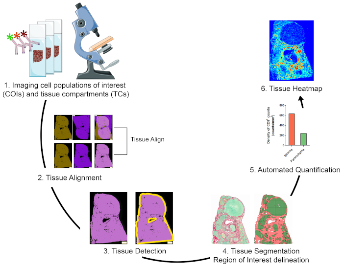
Figure 1: Schematic representation of the strategy for visualizing, quantifying, and mapping immune cells in the TME. (1) Serial whole tissue sections were stained for labeling COIs and TCs. Stained whole tissue sections were digitized using a whole slide scanner. (2) Images acquired from serial sections were linked, aligned, and coregistered in an automated fashion using a Tissuealign analysis module. A composite image was generated from the high-precision alignment of individual images. (3) A user-defined protocol was used for automated detection of tissue-associated pixels (TAPs) in the composite image. (4) The tissue was segmented into TCs (e.g., stroma and parenchyma) defined as ROIs. (5) User defined protocols were used for the automated detection and quantification of COIs in different TCs. (6) Tissue heatmaps of COIs were generated. Please click here to view a larger version of this figure.

Imaging COIs and TCs
Three serial FFPE whole tissue sections of resected tumor from a subject with HBV-associated hepatocellular carcinoma were stained in one or more rounds of staining as in Figure 2A. Section I was stained with H&E to show the tissue architecture, cell morphology, and to determine clinically relevant parameters such as type of malignancy, tumor grade, and overall assessment of immune infiltration (Figure 2C). In contiguous section II, two rounds of mIF were used for labeling liver parenchymal and non-parenchymal cells (Figure 2A). In the first round, normal and tumor vessels were visualized using CD34 staining of endothelial cells. Additionally, epithelial cells (hepatocytes and cholangiocytes) were identified using cytokeratin 8/18, and fibrogenic activated hepatic stellate cells were identified as alpha smooth muscle actin positive (αSMA+) cells (Figure 2C). Following image acquisition, tissue sections were stripped and reprobed with antibodies against macrophages (CD68), and myofibroblasts (desmin). To better characterize the tumor immune infiltrate, adjacent serial section III was stained using two rounds of mIF for the cellular markers CD3, CD4, CD8, forkhead box P3 (FoxP3), and myeloperoxidase (MPO). In all cases DAPI was used as a nuclear counterstain. Finally, section III was stained with PSR stain and counterstained with fast green to visualize fibrillar collagen and segment the tissue into stroma and parenchyma (Figure 2C).

A whole slide scanner equipped with a 20X objective lens was used to digitize stained sections and to create virtual slides. Six images were acquired from the three serial sections (Figure 2B) and the virtual slides subsequently analyzed using the VIS software according to the schematic representation in Figure 1.

Image Analysis
The image analysis comprised five steps: 1) tissue alignment; 2) tissue detection; 3) tissue segmentation; 4) automated quantification of COIs; and 5) tissue heat mapping. All protocols for image analysis were developed using the Author module of the image analysis software and are referred to in the text as APP.

Tissue alignment
Six virtual slides from three serial sections, spanning 11 markers plus H&E and PSR stains, were loaded into the Tissualign module of the image analysis software. Next, the images were linked, aligned, and coregistered in an automated fashion, generating an 11-plex plus H&E and PSR virtual composite image, containing all the layers of the individual images (Figures 2A–C). Alignment was accurate in the case of images originating from adjacent serial sections, showing corresponding tissue structures positioned and arranged in a homologous fashion upon alignment (Figure 2C and Figure S1A). Furthermore, the alignment was precise at the individual cell level for images originating from the same section (Figure S1B). The time for automatic alignment depends on the number, size, complexity, and similarity of the images to be aligned. The alignment of the above-mentioned six virtual slides took 15 min in our VIS station.

Figure 2: Staining of serial tissue sections and image alignment. (A) Summary of stainings done on three serial sections for visualization of COIs and TCs. Numbers in brackets indicate image designation. For sections II and III, tissues were stripped and reprobed with a second cocktail of antibodies. (B) Overview of six individual whole tissue images before and after tissue alignment (left and right, respectively). Scale bar = 3,500 µm. (C) Zoomed view of aligned images. Scale bar = 80 µm. Please click here to view a larger version of this figure.

Tissue Detection
Once the images were linked and aligned, we sought to identify the TAPs (Figure 3A). To design an APP for the automated detection of TAPs (APP 1, Table 1), we took advantage of two properties that differentiate TAPs from pixels not associated with tissue. First, the DAPI signal (blue band) is restricted to the nuclei, which are located exclusively in the tissue, meaning that all DAPI+ pixels are a subset of TAPs. Second, TAPs have higher autofluorescence signal in the green and yellow bands compared to pixels not associated with the tissue. Consequently, we developed APP 1 for tissue detection (Table 1), which detects the TAPs based on baseline signal in these channels using simple thresholding techniques. Thresholds for the blue, green, and yellow bands were set so that TAPs had background intensity values above the thresholds, while pixels not associated with the tissue had values below. APP 1 for tissue detection was applied to image IIA, which contains layers in the blue, green, and yellow channels (Figure 3A). As outputs of APP 1, a bright green mask was laid down on top of the TAPs, and a ROI called "Tissue" was delineated (output, Figure 3A). Furthermore, the area of the tissue was determined as a quantitative output variable. Because APP 1 does not incorporate the pixels not associated with the tissue into the ROI Tissue, they were excluded from subsequent analysis based on this ROI (Figure 3A). The precision of APP 1 at identifying TAPs is shown in Figure 3A.

Tissue segmentation and delineation of ROIs for TCs
Next, we proceeded to define different compartments inside the ROI tissue by segmenting the tissue into stroma versus parenchyma. We used the PSR stained image (IIIC, Figure 2C), where the stroma can be defined as the area associated with the deposition of fibrillar collagens (red band), the parenchyma as the area where fibrillar collagens are absent, and the fast green counterstaining dye prevails (green band) (Figure 3B). We created APP 2 (Table 1) to digitally delimit the TCs Stroma and Parenchyma. This APP works on the predefined ROI Tissue (output, Figure 3A) and uses representative stroma and parenchyma areas for training the Classifier tool integrated in the Image Analysis module. The trained Classifier assigns the pixels to either a stroma or a parenchyma label (salmon and green, respectively, Figure 3B). Upon classification of pixels, APP 2 executed morphological operations aiming at defining the ROIs Stroma and Parenchyma (Figure 3B and Table 1). The performance of APP 2 at classifying pixels and generating the respective ROIs is shown in Figure 3B. Additionally, APP 2 quantifies the area of the stroma and the parenchyma. Finally, even though the segmentation is done using the PSR stained section, the outlined stroma and parenchyma regions can be transferred to any image aligned to the PSR image.

Figure 3: Automated tissue detection/segmentation and generation of respective ROIs. (A) Image IIA was used to identify the TAPs (left image, scale bar = 6,000 µm). A bright green mask was assigned to the TAPs using APP 1 (Table 1) generating a ROI called Tissue (output 1). Right, inset shows zoomed view demonstrating the precision of APP 1 at detecting TAPs. Scale bar = 350 µm. (B) The ROI Tissue (output 1) is segmented into stroma and parenchyma using APP 2. The image on the left shows a view of the ROI Tissue segmented into ROI stroma (salmon) and ROI parenchyma (green). Scale bar = 4,500 μm. On the right, zoomed views of inset for ROI Tissue, the original PSR staining (image IIIC), and the ROIs stroma and parenchyma. Scale bar = 250 μm. Please click here to view a larger version of this figure.

Automated quantification of COIs
Next, we proceeded to identify, locate, and quantify COIs in the ROIs Stroma and Parenchyma. APPs 3 to 8 (Table 1) were created to locate and count the following COIs: CD4+FoxP3+, CD8+, CD68+, MPO+, αSMA+, and CD34+ cells, respectively. APP 3 was designed to locate and count CD4+FoxP3+ cells (image IIIA, Figure 2C) as surrogate markers of regulatory T cells (Tregs). This protocol detects colocalization of the signal from the nuclear transcription factor FoxP3 (red band) and the DNA labeling dye DAPI (blue band). Given that recently activated T cells upregulate FoxP3, to enrich for Tregs we set thresholds for preselecting only bright FoxP3+ cells (FoxP3^hi). Next, out of all preselected DAPI+FoxP3^hi cells, only those that were surrounded by bright ring-shaped CD4 signals (green band) were labelled and counted as FoxP3^hiCD4+ cells (pink label, Figure 4A). The density of FoxP3^hiCD4+ cells in the ROIs Stroma and Parenchyma were determined as quantitative output variables of APP 3 (Figure 4A).

Similarly, APPs 4 to 6 were designed for the detection of CD8+, CD68+, and MPO+ cells. These APPs share the same baseline design for detecting and quantifying COIs. Specifically, COIs are identified based on signal intensity from the specific cell population biomarker, and then several postprocessing morphological steps are executed to delineate individual cells (Table 1). The individual cells or COIs are labelled, counted, and their tissue coordinates registered. APPs 4 to 6 also determine the density of the COIs in the ROIs Stroma and Parenchyma (Figure 4B–D).

The quality of our DAPI staining was not good enough for integrating nuclei segmentation into APPs 3 to 6, so we cannot ensure that all individually labelled objects are individual cells. For this reason, we expressed the density of cells in counts of labeled objects/mm² (Figure 4). However, cell aggregates were successfully separated into individual cells in the postprocessing steps built into APPs 3 to 6, and extensive visual inspection showed that most labeled objects corresponded to single cells.

For detecting αSMA+ and CD34+ area, we developed APPs 7 and 8, respectively (Table 1). Both APPs detect the specific signal based on thresholds and determine the percentage of positive area in the ROIs Stroma and Parenchyma (Figure 4E–F).

One of the most interesting possibilities of generating virtual multiplex slides is the analysis of colocalization expression. We generated APP 10 to detect colocalization between αSMA and desmin, two markers co-expressed by myofibroblasts in the liver. APP 10 uses thresholds for finding pixels positive for αSMA, desmin, and αSMA plus desmin (Table 1). As quantitative output variables, APP 10 determines the αSMA+ area, the desmin+ area, and the area of colocalized expression of these two markers (Figure S3).

Figure 4: Identification and quantification of COIs in the TCs stroma and parenchyma. (A–F) Automated detection and quantification of CD4+FoxP3+, CD8+, CD68+, MPO+, αSMA+, and CD34+ COIs in the ROIs Stroma and Parenchyma using protocols 3, 4, 5, 6, 7, and 8, respectively (Table 1). Shown on the left are the original images, in the middle the processed images, and on the right the quantifications. For Figures 4A–D, scale bar = 40 µm. For Figures 4E and F, scale bar = 350 µm. Please click here to view a larger version of this figure.

As an alternative to quantifying the COIs in the TCs Stroma and Parenchyma, we determined the density of immune cells in the different malignant nodules named 1 to 4 (Figure 5A, H, and I). The ROI for each nodule was manually delineated as indicated in Figure 5A. Distinctive tissue immune signatures characterized each nodule, further revealing the intrinsic heterogeneity of the TME.

Tissue Heatmaps
As mentioned above, APPs 3 to 8 store the tissue coordinates of every individually labelled object. This feature allows the automated generation of tissue maps where regions of high density of a given cell population are displayed as hot spots (red), and regions with relatively low density as cold spots (dark blue). Intermediate density values are assigned colors according to the color scale shown in Figure 5. Tissue heatmaps were generated by APPs that divided the images into circles of 50 μm diameter and assigned a color according to the relative density of a given COI inside the circle. As displayed in Figure 5B–G, the positioning patterns and intensity distribution of the different COIs in the TME was quite varied. Furthermore, at the level of individual nodules, the arrangement of different populations in the tissue area was unique (Figure S2A–C). To provide an example of the power of this technique and to visualize the spatial organization of hot spots from different populations in the same nodule, the hot spots from individual cell types were manually extracted and mapped together onto the outline of nodule 2 (Figure S2, Figure D, and Figure E).

Figure 5: Tissue heatmaps of COIs in the TME. (A) Picrosirius Red staining showing location of nodules 1, 2, 3, and 4. (B–G) Tissue heatmaps for CD4+FoxP3+, CD8+, CD68+, MPO+, CD34+, and αSMA+ COIs, respectively. Dark blue indicates relative low density, and red indicates relative high density. Intermediate density values are assigned colors according to the shown color scale. (H and I) Quantification of COIs in nodules 1, 2, and 3 + 4 organized per cell type and per nodule, respectively. Please click here to view a larger version of this figure.

Supplementary Figure S1: Validation of tissue alignment. (A) CD34 staining (in red) done on section II (input 1) is used for generating a CD34 mask in green (output 1). The green mask (output 1) is overlaid on the H&E image from the aligned serial section I (input 2). The merge image shows perfect correspondence of vascular structures. Scale bar = 50 μm. (B) Image IIIA showing the merge of DAPI, CD4, and FoxP3 (input 1) was used to generate a label for CD4+FoxP3+ cells (output 1 in magenta). Output 1 label was transferred onto aligned image IIIB (input 2) and shows perfect correspondence between the pairs FoxP3/DAPI, and CD4/CD3 in the merge image. Scale bar = 15 μm. Please click here to view a larger version of this figure.

Supplementary Figure S2: Zoomed view of tissue heatmaps. (A–C) Tissue heatmaps for CD4+FoxP3+, CD8+, CD68+, and MPO+ cells in nodules 1–4. Scale bars in nodules 1, 2, and 3 + 4 represent 1,500 μm, 700 μm, and 500 μm respectively. (D) Outline of nodule 2 with black solid line. (E) Hot spots for CD4+FoxP3+, CD8+, CD68+, and MPO+ cells in nodule 2 were extracted and mapped together onto the nodule 2 outline defined in D. Please click here to view a larger version of this figure.

Supplementary Figure S3: Colocalization Analysis. (A) On the left and middle are images of αSMA label in green and desmin label in red respectively. On the right is a αSMA/desmin double positive area in yellow. (B) Quantification of αSMA+ area, desmin + area, and αSMA/desmin double positive area. Scale bar = 150 μm. Please click here to view a larger version of this figure.

APP	Purpose	Classification	Classification	Post-Processing Steps	Output Variables
		Method	Features
			(pixel value)
1	Tissue detection	Threshold	Channel DAPI (150)	o Label objects with colocalized above-threshold values for the 3 channels	o ROI Tissue
			Channel FITC/A488 (120)	o Close positive object 5 pixels	o Tissue Area
			Channel TRITC/A568 (40)	o Create ROI Tissue
2	Tissue Segmentation	Decision Forest	RGB-R median	o Fill holes	o ROI Stroma
			RGB-G median	o Create ROI Stroma	o Stroma Area
			RGB-B median	o Create ROI Parenchyma	o ROI Parenchyma
			IHS-S median		o Parenchyma Area
			H&E Eosin median
3	To locate and quantify CD4+ FoxP3+ cells	Threshold	Channel DAPI (>600)	o Label objects with colocalization of DAPI and Cy5/A647, surrounded by FITC/A488 signal	o Counts and density of CD4+FoxP3+ cells in ROIs Stroma and Parenchyma
			Channel FITC/A488 poly smoothing (>850)	o Clear objects smaller than 7 μm2	o Coordinates of individual CD4+FoxP3+ cells
			Channel Cy5/A647(>800)
4	To locate and quantify CD8+ cells	Threshold	Channel DAPI (<1200)	o Clear positive objects smaller than 15 μm2	o Counts and density of CD8+ cells in ROIs Stroma and Parenchyma
			Channel Cy5/A647 median (>80)	o Close positive objects 2 pixels	o Coordinates of individual cells
				o Separate objects
5	To locate and quantify CD68+ cells	Threshold	Channel FITC/A488 (>200)	o Clear positive objects smaller than 20 μm2	o Counts and density of CD68+ cells in ROIs Stroma and Parenchyma
				o Dilate positive objects 3 pixels	o Coordinates of individual CD68+ cells
				o Separate objects
6	To locate and quantify MPO+ cells	Threshold	Channel DAPI (>400)	o Clear objects smaller than 5 μm2	o Counts and density of MPO+ cells in ROIs Stroma and Parenchyma.
			Channel TRITC/A568 (900-4000)	o Dilate 3 pixels positive objects	o Coordinates of individual MPO+ cells.
				o Separate objects
7	To locate and quantify αSMA+ area	Threshold	Channel TRITC/CF568 (>1050)	o Clear positive objects smaller than 25 μm2	o Counts and density of αSMA+ area in ROIs Stroma and Parenchyma
				o Dilate 3 pixels positive objects	o Coordinates of αSMA+ pixels
8	To locate and quantify CD34+ area	Threshold	Channel DAPI (<5000)	o Clear positive objects smaller than 25 μm2	o Counts and density of CD34+ area in ROIs Stroma and Parenchyma
			Channel Cy5/A647 median (>120)	o Dilate 3 pixels positive objects	o Coordinates of CD34+ pixels
9	Create tissue heatmaps for a given cell population	Object Heatmap	Object Heatmap		o Heatmap
			Drawing radius 50 μm	---
10	Quantify colocalization between αSMA and Desmin	Threshold	Channel TRITC (CF568) (>1050)	o Label objects with above threshold values for TRITC (CF568)	o Quantify colocalized expression of αSMA and Desmin
			Channel Cy5 (A647) (>1000)	o Label objects with above threshold values for Cy5 (A647)
				o Label objects with colocalization of above threshold values for TRITC (CF568) and Cy5 (A647)
				o Clear positive objects smaller than 25 μm2

Table 1: General parameters used for the design of APPs employed for image analysis. The parameters specified in this table are adjusted to the unique characteristics of the images used in this analysis (e.g., background, artifacts, etc.) and may not be applicable to other images. Because the post-processing steps mentioned were defined for the specific images analyzed in this study, they are intentionally not detailed. The user should customize the APPs to the images to be analyzed.

Section/Staining	Primary Antibody	Secondary Antibody
Section II/1st Staining	Mouse IgG2a anti-human αSMA Mouse IgG1 anti-human CD34 Rabbit anti-human Cytokeratin 8/18	Goat anti-mouse IgG2a CF568 Rat anti-mouse IgG1 A647 Donkey anti-rabbit A488
Section II/2nd Staining	Rabbit anti-human Desmin Mouse anti-human CD68	Donkey anti-rabbit A647 Donkey anti-mouse DyLight 755
Section III/1st Staining	Mouse anti-human CD4 Rabbit anti-human FoxP3 Goat anti-human MPO	Donkey anti-mouse A488 Donkey anti-rabbit A647 Donkey anti-goat A568
Section III/2nd Staining	Rabbit anti-human CD3 Mouse anti-human CD8	Donkey anti-mouse DyLight 755 Donkey anti-rabbit A647

Table 2: Primary-Secondary Antibody Pairs for mIF.

Discussion

Simple, accessible, and easy to execute multiplexing techniques that allow spatial resolution of immune cells in tissue sections are needed to map the immune landscape in cancer and other immunological disorders. Here, we describe a strategy that integrates widely available labeling and digital analysis techniques to expand the multiplexing capability and multidimensional assessment of imaging assays^12,13,17,19. The staining of three serial sections for different markers, and the reuse of sections through stripping and reprobing techniques, enabled us to visualize 11 parameters in addition to H&E and PSR stains. Six images from these sections were aligned in an automated fashion using the tissue alignment module. The alignment was precise at the individual cell level for images originating from the same section and highly concordant for images originating from neighboring sections. Virtual multiplexing enabled us to determine how markers visualized in one section relate spatially to markers visualized in another contiguous section. While some of the stainings labelled COIs, others labelled TCs, allowing us to quantify COIs in the different TCs. The use of software tools for the automated quantification of COIs greatly simplified and accelerated the processing of images. Moreover, digital analysis was applied to whole tissue sections instead of selected fields of view, resulting in an unbiased representation of the TME. Furthermore, because the tissue coordinates of COIs were registered, it was possible to generate tissue heatmaps.

There are several areas in this protocol where troubleshooting may be needed. First, poor antigen retrieval can affect the quality of mIF, therefore the type of antigen retrieval buffer and duration should be optimized for the specific assay/biomarker conditions used. Second, the type of blocking solution used should be adapted to the tissues/antigen/species of primary and secondary antibodies. In our hands, the addition of 10% total serum from the species where the tissue comes from blocked Fc receptors, and thus reduced nonspecific antibody binding. Addition of 10% of serum from the species the secondary antibodies were raised in would minimize direct nonspecific attachment of secondary antibodies to the tissue section. Third, validation of the specificity of the primary and secondary antibodies using the proper positive and negative controls is essential. Fourth, increased autofluorescence in some channels and diffusion of DAPI upon primary antibody stripping are also common. To address the enhanced autofluorescence, we used primary/secondary antibody pairs where the specific signal had intensity values at least 5x that of the background. Finally, some high affinity antibodies cannot be eluted with regular stripping procedures. In this case, we recommend using such antibodies in the last round of labeling. The user may have to try different staining sequences to find the optimal configuration for the antibodies of interest. Efficiency of stripping should be confirmed before proceeding to a second or third round of labeling.

The main limitation and challenge of this strategy is finding the right combinations of primary and secondary fluorescent antibodies for the markers of interest. Finding primary antibodies raised in different species or with different isotypes that could be used simultaneously is limited by what is commercially available. Most whole slide scanners are equipped with lamps and filters that allow imaging a maximum of five channels, and secondary antibodies in the right species and right fluorophore are not always available. We partially overcame these limitations using serial stainings and sequential labeling. Several antibody combinations may need to be tested to arrive at the best combination for the markers of interest. Another limitation is the quality of the DAPI staining, because stripping and reprobing may not always allow performing nuclei segmentation.

The tissue align module requires minimal training and no programming skills from users. The software theoretically allows alignment of an unlimited number of images. However, precise alignment depends on relatedness of sections, where closer sections that are more histologically concordant are more accurately aligned. We used the Author module of VIS for generating the APPs. Basic knowledge of image analysis is needed for creating APPs, but this is equally the case when using any other image analysis software. The unique advantages of VIS as compared to other image analysis software include automated alignment of images from sections prepared using different methods (e.g., IF, histochemistry, IHC). This allows colocalization studies of multiple markers of interest using virtual multiplexing. Furthermore, the flexible and user-friendly design of APPs allows user-specific customization. Automated quantification and mapping, and the possibility of processing whole tissue sections, saves time and reduces bias compared to manual counting by visual inspection.

This strategy is a very useful research tool for tissue immunology in the context of cancer and autoimmunity but remains unvalidated for clinical use. With additional standardization and validation, it can be used in the future for multiple applications (e.g., to map the immune landscape in cancer to predict and monitor the response to immunotherapeutic agents). It can also be adapted to different inflammatory conditions (e.g., inflammatory bowel disease) to combine pathological evaluation with prognostic biomarkers.

The main critical steps in this protocol are the efficiency/specificity of the labeling and the robustness of the designed APPs for the intended use or biomarker. Hence, regular validation by visual inspection, especially upon designing a new APP, is essential. The efficient use of multiple rounds of stripping and reprobing or different types of stains on the same section are critical components and can be tissue or section specific. Verifying the efficiency of such processes before proceeding with large batch analysis is critical.

In summary, we provide a strategy that maximizes the quantitative and spatial information that can be obtained from valuable clinical tissue samples. The resources, equipment, and knowledge required to implement this methodology are widely accessible. We propose this methodology as a useful guide for planning assays aiming at identifying, quantifying, and mapping immune cell populations in the TME.

Materials

Name	Company	Catalog Number	Comments
Antigen Retrieval Solution: Sodium Citrate Buffer (10 mM Sodium Citrate, 0.05% v/v Tween 20, pH 6.0)
Blocking Solution: 1 % BSA, 10 % filtered human serum, 10 % filtered donkey serum, 0.1 % Tween 20, and 0.3% Triton in PBS
Bovine serum albumin (BSA)	Multicell	800-095-EG
Coplin jars (EASYDIP SLIDE STAINING SYSTEM)	Newcomersupply	5300KIT
Cover slides	Fisherbrand	12-545E 22*50
Direct Red 80	Sigma Aldrich	365548
Donkey Serum	Sigma Aldrich	D9663
Ethanol 100%
Electric pressure cooker	Salton
Eosin	Leica Biosystems	3801600	CAUTION, eye irritation
Fast Green FCF	Sigma Aldrich	F7252	CAUTION, harmful by inhalation, ingestion and skin absortion
FFPE section (4μm) slides
Glycine 0,1 M in PBS
Hematoxylin Stain Solution, Gil 1. Formulation, Regular Strength	Ricca Chemical Company	3535-32
Holder (EasyDip Staining Jar Holder)	Newcomersupply	5300RK
Human Serum	Gemini	22210
Humidity chamber	Millipore Sigma	Z670138-1EA
Pap pen	abcam	ab2601
PBS
PBS-Tween 20 (0.1% v/v)
Permount Mounting Media	Fisher Chemical	SP15-500
Picric Acid 1.3 %	Sigma Aldrich	P6744	CAUTION, skin and eye irritation
Picro-Sirius Red/Fast Green solution: Fast Green 0.1 % w/v + Sirius Red 0.2 % w/v in 1,3 % picric acid solution
Primary Antibody Anti-αSMA	Mouse IgG2a 1A4	Sigma A2547	Dilution 1/100
Primary Antibody Anti-CD34	Mouse IgG1 HPCA1/763	Novus Biologicals NBP2-44568	Dilution 1/250
Primary Antibody Anti-Cytokeratin 8/18	Rabbit EP17/EP30	Agilent IR09461-2	Ready to use
Primary Antibody Anti-CD68	Mouse KP1	Abcam ab955	Dilution 1/200
Primary Antibody Anti-Desmin	Rabbit Polyclonal	Invitrogen PA5-16705	Dilution 1/200
Primary Antibody Anti-CD4	Mouse N1UG0	Affymetrix 14-2444	Dilution 1/250
Primary Antibody Anti-FoxP3	Rabbit 1054C	R & D MAB8214	Dilution 1/100
Primary Antibody Anti-MPO	Goat Polyclonal	R & D Systems AF3667	Dilution 1/250
Primary Antibody Anti-CD3	Rabbit SP7	Abcam ab16669	Dilution 1/200
Primary Antibody Anti-CD8	Mouse C8/144B	Invitrogen 14-0085-80	Dilution 1/200
Secondary Antibody Donkey anti-mouse A488	Polyclonal	Invitrogen A-21202	Dilution 1/500
Secondary Antibody Donkey anti-Rabbit A488	Polyclonal	Invitrogen A-21206	Dilution 1/500
Secondary Antibody Donkey anti-goat A568	Polyclonal	Invitrogen A-11057	Dilution 1/500
Secondary Antibody Donkey anti-rabbit A647	Polyclonal	Invitrogen A-31573	Dilution 1/500
Secondary Antibody Rat anti-mouse IgG1 A647	RMG1-1	Biolegend 406618	Dilution 1/500
Secondary Antibody Goat anti-mouse IgG2a CF568	Polyclonal	Sigma Aldrich SAB4600315	Dilution 1/500
Secondary Antibody Donkey anti-mouse DyLight 755	Polyclonal	Invitrogen SA5-10171	Dilution 1/500
Secondary Antibody Donkey anti-rabbit DyLight 755	Polyclonal	Invitrogen SA5-10043	Dilution 1/500
SDS	BioShop	SDS001,500	CAUTION, oral skin and eye toxicity
Shandon multi-program robotic slide stainer	LabX	11384903
Shandon Xylene Substitute,	Thermo Fisher Scientific	CA89413-336	CAUTION, Flammable, skin and eye irritation, Harmful when inhaled
Shaking water bath
SlowFade Gold antifade reagent with DAPI	Invitrogen	S36938
Sodium Citrate Dihydrate	Millipore Sigma	1545801	CAUTION, eye irritation
Stripping Buffer: mix 20 ml 10% w/v SDS with 12.5 ml 0.5 M Tris-HCl (pH 6.8), and 67.5 ml ultra-pure water. Under a fume hood, add 800 uL of 2-mercapto ethanol (114,4 mM final concentration)
Triton X-100	Sigma Aldrich	T8787-50ML
Tris-HCl	BioShop	77-86-1
Tween 20	Fisher Scientific	BP337-500
VIS Software	Visiopharm
Whole slide scanner Olympus BX61VS	Olympus		Microscope: Olympus Slide Scanner BX61VS, 5 slides scanner, motorized stage, autofocus. Camera: Lightsource: Xcite-120. Filters: BrightLine® Sedat filter set (# LED-DA/FI/TR/Cy5-4X4M-B-000, Semrock)
Xylene	Sigma Aldrich	214736-4L	CAUTION, Flammable, skin and eye irritation, Harmful when inhaled
Xylene : Ethanol solution (1:1 v/v)
2-mercaptoethanol	Sigma	M6250	CAUTION, harmful by ingestion, inhalation, fatal if sking absortion. Eye irritation. Use fume hood

References

- Greten, F. R., Grivennikov, S. I. Inflammation and Cancer:Triggers, Mechanisms, and Consequences. Immunity. 51 (1), 27-41 (2019).
- Pages, F., et al. International validation of the consensus Immunoscore for the classification of colon cancer: a prognostic and accuracy study. Lancet. 391 (10135), 2128-2139 (2018).
- Binnewies, M., et al. Understanding the tumor immune microenvironment (TIME) for effective therapy. Nature Medicine. 24 (5), 541-550 (2018).
- Taube, J. M., et al. Implications of the tumor immune microenvironment for staging and therapeutics. Modern Pathology: an official journal of the United States and Canadian Academy of Pathology, Inc. 31 (2), 214-234 (2018).
- Bindea, G., et al. Spatiotemporal dynamics of intratumoral immune cells reveal the immune landscape in human cancer. Immunity. 39 (4), 782-795 (2013).
- Galon, J., et al. Towards the introduction of the 'Immunoscore' in the classification of malignant tumours. The Journal of Pathology. 232 (2), 199-209 (2014).
- Finotello, F., Eduati, F. Multi-Omics Profiling of the Tumor Microenvironment: Paving the Way to Precision Immuno-Oncology. Frontiers in Oncology. 8, 430 (2018).
- Gerner, M. Y., Kastenmuller, W., Ifrim, I., Kabat, J., Germain, R. N. Histo-cytometry: a method for highly multiplex quantitative tissue imaging analysis applied to dendritic cell subset microanatomy in lymph nodes. Immunity. 37 (2), 364-376 (2012).
- Giesen, C., et al. Highly multiplexed imaging of tumor tissues with subcellular resolution by mass cytometry. Nature Methods. 11 (4), 417-422 (2014).
- Porta Siegel, T., et al. Mass Spectrometry Imaging and Integration with Other Imaging Modalities for Greater Molecular Understanding of Biological Tissues. Molecular Imaging and Biology : MIB: the official publication of the Academy of Molecular Imaging. 20 (6), 888-901 (2018).
- Buchberger, A. R., DeLaney, K., Johnson, J., Li, L. Mass Spectrometry Imaging: A Review of Emerging Advancements and Future Insights. Analytical Chemistry. 90 (1), 240-265 (2018).
- Pirici, D., et al. Antibody elution method for multiple immunohistochemistry on primary antibodies raised in the same species and of the same subtype. Journal of Histochemistry and Cytochemistry. 57 (6), 567-575 (2009).
- Gendusa, R., Scalia, C. R., Buscone, S., Cattoretti, G. Elution of High-affinity (>10-9 KD) Antibodies from Tissue Sections: Clues to the Molecular Mechanism and Use in Sequential Immunostaining. Journal of Histochemistry and Cytochemistry. 62 (7), 519-531 (2014).
- van der Loos, C. M. Multiple immunoenzyme staining: methods and visualizations for the observation with spectral imaging. Journal of Histochemistry and Cytochemistry. 56 (4), 313-328 (2008).
- Stack, E. C., Wang, C., Roman, K. A., Hoyt, C. C. Multiplexed immunohistochemistry, imaging, and quantitation: a review, with an assessment of Tyramide signal amplification, multispectral imaging and multiplex analysis. Methods. 70 (1), 46-58 (2014).
- Toth, Z. E., Mezey, E. Simultaneous visualization of multiple antigens with tyramide signal amplification using antibodies from the same species. Journal of Histochemistry and Cytochemistry. 55 (6), 545-554 (2007).
- Robertson, D., Savage, K., Reis-Filho, J. S., Isacke, C. M. Multiple immunofluorescence labeling of formalin-fixed paraffin-embedded (FFPE) tissue. BMC Cell Biology. 9, 13 (2008).
- Segnani, C., et al. Histochemical Detection of Collagen Fibers by Sirius Red/Fast Green Is More Sensitive than van Gieson or Sirius Red Alone in Normal and Inflamed Rat Colon. PloS One. 10 (12), 0144630 (2015).
- Bolognesi, M. M., et al. Multiplex Staining by Sequential Immunostaining and Antibody Removal on Routine Tissue Sections. Journal of Histochemistry and Cytochemistry. 65 (8), 431-444 (2017).