Isolation and Time-Lapse Imaging of Primary Mouse Embryonic Palatal Mesenchyme Cells to Analyze Collective Movement Attributes

Summary

We present a protocol for isolation and culture of primary mouse embryonic palatal mesenchymal cells for time-lapse imaging of two-dimensional (2D) growth and wound-repair assays. We also provide the methodology for analysis of the time-lapse imaging data to determine cell-stream formation and directional motility.

Abstract

Development of the palate is a dynamic process, which involves vertical growth of bilateral palatal shelves next to the tongue followed by elevation and fusion above the tongue. Defects in this process lead to cleft palate, a common birth defect. Recent studies have shown that palatal shelf elevation involves a remodeling process that transforms the orientation of the shelf from a vertical to a horizontal one. The role of the palatal shelf mesenchymal cells in this dynamic remodeling has been difficult to study. Time-lapse-imaging-based quantitative analysis has been recently used to show that primary mouse embryonic palatal mesenchymal (MEPM) cells can self-organize into a collective movement. Quantitative analyses could identify differences in mutant MEPM cells from a mouse model with palate elevation defects. This paper describes methods to isolate and culture MEPM cells from E13.5 embryos-specifically for time-lapse imaging-and to determine various cellular attributes of collective movement, including measures for stream formation, shape alignment, and persistence of direction. It posits that MEPM cells can serve as a proxy model for studying the role of palatal shelf mesenchyme during the dynamic process of elevation. These quantitative methods will allow investigators in the craniofacial field to assess and compare collective movement attributes in control and mutant cells, which will augment the understanding of mesenchymal remodeling during palatal shelf elevation. Furthermore, MEPM cells provide a rare mesenchymal cell model for investigation of collective cell movement in general.

Introduction

Palate development has been studied extensively as defects in palatogenesis lead to cleft palate-a common birth defect that occurs in isolated cases or as part of hundreds of syndromes^1,2. The development of the embryonic palate is a dynamic process that involves movement and fusion of embryonic tissue. This process can be divided into four major steps: 1) induction of palatal shelves, 2) vertical growth of the palatal shelves next to the tongue, 3) elevation of the palatal shelves above the tongue, and 4) fusion of the palatal shelves at the midline^1,3,4. Over the past several decades, many mouse mutants have been identified that manifest cleft palate^5,6,7,8. Characterization of these models has indicated defects in palatal shelf induction, proliferation, and fusion steps; however, palatal shelf elevation defects have been rare. Thus, understanding the dynamics of palatal shelf elevation is an intriguing area of research.

Careful analysis of some mouse mutants with palatal shelf elevation defects has led to the current model showing that the very anterior region of the palatal shelf appears to flip up, while a vertical to horizontal movement or "remodeling" of the palatal shelves occurs in the middle to posterior regions of the palate^{1,3,4,9,10,11}. The medial edge epithelium of the palatal shelf likely initiates the signaling required for this remodeling, which is then driven by the palatal shelf mesenchyme. Recently, many researchers have identified palatal shelf elevation delay in mouse models that showed transient oral adhesions involving palatal shelves^12,13. The mesenchymal remodeling involves reorganization of the cells to create a bulge in the horizontal direction, while simultaneously retracting the palatal shelf in the vertical direction^9,10,14. Among the several mechanisms proposed to affect palatal shelf elevation and the underlying mesenchymal remodeling are cell proliferation^15,16,17, chemotactic gradients¹⁸, and extracellular matrix components^19,20. An important question arose: is the palatal shelf elevation delay observed in Specc1l-deficient mice also partly due to a defect in the palatal shelf remodeling, and could this remodeling defect manifest in an intrinsic defect in behavior of primary MEPM cells²¹?

Primary MEPM cells have been used in the craniofacial field for many studies involving gene expression^{22,23,24,25,26,27,28,29}, and a few involving proliferation^30,31 and migration^25,31,32, but none for collective cell behavior analysis. Time-lapse imaging of MEPM cells was performed in 2D culture and wound-repair assays to show that MEPM cells displayed directional movement and formed density-dependent cell streams-attributes of collective movement²¹. Furthermore, Specc1l mutant cells formed narrower cell streams and showed highly variable cell migration trajectories. This lack of coordinated motility is considered to contribute to the palate elevation delay in Specc1l mutant embryos^13,21. Thus, these relatively simple assays using primary MEPM cells may serve as a proxy for studying mesenchymal remodeling during palatal shelf elevation. This paper describes the isolation and culture of primary MEPM cells, as well as the time-lapse imaging and analysis, for the 2D and wound-repair assays.

Protocol

All experiments involving animals were carried out with a protocol approved by the KUMC Institutional Animal Care and Use Committee, in accordance with their guidelines and regulations (Protocol Number: 2018-2447).

1. Harvest E13.5 embryos

1. Euthanize pregnant female mice using a CO₂ inhalation chamber or by a procedure approved by the Institutional Animal Care and Use Committee. Immediately proceed to dissection.
2. Expose the inferior half of the abdominal cavity by removing the skin and peritoneum. Excise both horns of the uterus, which contain the E13.5 embryos.
3. Briefly place the uterus in prewarmed 37 °C sterile phosphate-buffered saline (PBS) to rinse off excess blood, hair, or other debris. Place the uterus in a sterile 10 cm dish filled with sterile PBS.
4. Using small scissors, cut through the uterine wall along the length of the uterus to expose each embryo, still in its yolk sac. Remove the yolk sac surrounding the embryo, but save it for genotyping, if needed. As the embryos are removed, place each embryo in its own well of a 12-well plate filled with PBS.

2. Dissection of palatal shelves from embryos (Figure 1)

NOTE: Sterilize the stainless steel dissection instruments (see the Table of Materials) after processing each embryo by placing the instruments first in a beaker of 100% ethyl alcohol (EtOH), then in an instrument sterilizer at 350 °C for 10 s, and then cooling them in a second beaker of 100% EtOH.

1. Using a sterilized perforated spoon, place the embryo in a new 10 cm dish filled with MEPM culture medium consisting of Dulbecco's minimum essential medium (DMEM) containing 10% fetal bovine serum (FBS), L-glutamine (4 mM L-Glu), and the antibiotics-penicillin and streptomycin (50 units/mL).
2. Decapitate the embryo right below the jaw line using sterile scissors (Figure 1A, red dotted line). Remove the lower jaw by inserting one point of the sterilized fine #5 forceps into the mouth, keeping it just inside the cheek. Push the point of the inserted forceps through until it exits out the back of skull.
3. Orient the forceps, along the yellow line in Figure 1B, so that the other side of the forceps (which is still outside of the embryo) is hovering just over the ear canal, then pinch the forceps shut to cut the tissue. If necessary, run another fine forceps along the seam of the now closed forceps to cut through any tissue that was not completely severed by the pinch.
4. Repeat the previous step for the other side of the embryo head. Continue the pinch-cut procedure to fully remove the lower jaw, tongue, and inferior portion of the skull and expose the palatal shelves.
5. Remove the cranium of the skull by cutting just above the eyes, as shown in Figure 1C (green line). Do this by placing the head on its left or right side and positioning the points of the small stainless steel scissors in front of and behind the skull just above the embryo's eye level. Cut off the top of the skull with one fast snip of the scissors, creating a flat surface that will be important for stability in later steps and that should look like Figure 1D when viewed from the side.
6. Place the remaining part of the head upside down, with the superior aspect of the head (cranium removed) resting flat on the bottom of the dish, which will provide a stable surface for palatal shelf removal. Take a moment to identify the palatal shelves, which are now exposed and facing up and will appear as two raised ridges on either side of a central groove in the anterior half of the head (Figure 1E).
7. Pin the remaining portion of the head to the dish to immobilize it while the shelves are removed. Do this by inserting one point of a fine forceps through the tissue near the nasal region of head, anterior to the palatal shelves, and insert the other point of the forceps through the base of the skull, posterior to the palatal shelves. Hold these in place while performing the excision of the palatal shelves.
   1. Immobilizing the head with one hand, pick any one of the two shelves to remove first, and insert both points of a second pair of fine forceps into the tissue at the base of the lateral surface of the shelf, and pinch to cut the tissue (Figure 1F). Repeat this along the base of the medial surface of the shelf and then at both the anterior and posterior ends of the shelf to detach from the head.
8. Gently lift the shelf, making additional pinches, as needed, to completely free the shelf from the surrounding tissue.
9. Repeat the previous two steps to remove the second palatal shelf.
10. With the palatal shelves now freed from the surrounding tissue and placed in PBS (Figure G), use a sterile plastic bulb transfer-pipette to draw up the shelves in the pipette, and transfer them into a 1.5mL microcentrifuge tube along with approximately 500 µL of PBS. Keep the tubes containing palatal shelves on ice as the rest of the litter is processed in the same fashion.
    NOTE: Alternatively, shelves can be placed in a 1.5mL microcentrifuge tube containing prewarmed trypsin (0.25%) immediately after dissection (in lieu of placing them on ice). Samples will be fresher, but care must be taken to time all the proceeding steps for each individual sample as opposed to treating the samples collectively.

3. Culture of MEPM cells

NOTE: Under the conditions described here, the palate epithelial cells do not survive the first passage, resulting in a pure palate mesenchymal cell culture. Use sterile technique to perform all steps in a tissue culture hood.

1. Aspirate and discard the PBS from the 1.5 mL tube, taking care not to discard the shelves in the process. Immediately add 200 µL of prewarmed (37 °C) trypsin (0.25%) to each tube that contains palatal shelves. Briefly pipet the shelves up and down in the trypsin using a 1000 µL pipette tip to accelerate the trypsinization.
2. Incubate the tubes for 5 min at 37 °C, then pipet each sample up and down again to help break up the tissue. Incubate the tubes for another 5 min at 37 °C, and pipet up and down once more to complete the dissociation of the tissue.
   NOTE: The shelves must be completely or nearly completely dissociated and suspended in the trypsin with no visible chunks of tissue remaining.
3. Add 800 µL of MEPM culture medium (step 2.1) to each 1.5 mL tube. Centrifuge the 1.5 mL tube at 200 × g for 5 min to pellet the cells. Remove the supernatant, and resuspend the cell pellet in 1 mL of MEPM culture medium.
4. Plate the MEPM cells into a 6-well tissue culture-treated plate containing MEPM culture medium. Allow the cells to adhere to the plastic surface for 12 h at 37 °C in an incubator with 5% CO₂.
   NOTE: After overnight incubation, the vast majority (~90%) of cells will attach. At this point, the adhered cells will look fairly homogeneous, with a triangular or slightly elongated shape.
5. Change the medium every day by gently aspirating the old medium and immediately replacing it with 1 mL of warm sterile PBS without calcium or magnesium for ~1 min. Aspirate the PBS, and replace with 3 mL of prewarmed MEPM culture medium.
6. Passage the cells once they become 100% confluent.
   NOTE: MEPM cells should proliferate by doubling in number almost daily.
   1. To passage the cells, gently aspirate the old medium, and immediately replace it with warm PBS without calcium or magnesium for ~1 min. Aspirate the PBS, and replace it with 0.5 mL of prewarmed 0.25% trypsin.
   2. Incubate at 37 °C for ~5 min, or until the cells detach from the surface of the dish when gently rocked back and forth by hand. Once the cells have detached, immediately add 5 mL of prewarmed MEPM culture medium to the trypsinized cells.
   3. Using a 10 mL serological pipet, gently collect the cells in a 15 mL conical tube, and centrifuge the tube at 200 × g for 5 min to pellet the cells. Aspirate the trypsin and medium, and resuspend the cells in 3 mL of prewarmed MEPM culture medium. Gently pipet 1 mL of cells into a single well of a 6-well dish, and add 2 mL of MEPM culture medium to bring the total volume to 3 mL.
      NOTE: This constitutes a 1:3 split of cells. MEPMs may be passaged up to three times. The seeding density of MEPMs is somewhat flexible, and the number of cells present varies depending on the culturing vessel. However, MEPMs do not properly proliferate when split too sparsely and should be at least 20-25% confluent in their new dish once they adhere.

4. Cryopreservation of MEPM cells

1. Once trypsinized MEPM cells are pelleted, resuspend the cells in MEPM culture medium to obtain a concentration of ~ 1 × 10⁶ cells/mL. Pipet the cells into cryovials, and add a final concentration of 5% dimethylsulfoxide in the cell stock. Cap the cryovial, briefly mix by inverting, and immediately place the vials in a freezing container that cools at a rate of 1 °C/min.
2. Place the cooler in a -80 °C freezer overnight. On the next day, move the cryovials to a liquid nitrogen tank for long-term storage.
3. Thawing cryopreserved MEPM cells
   1. Remove the cryovials from the liquid nitrogen tank, and thaw at room temperature until the contents begin to become liquid. Empty the contents into a 15 mL conical tube containing 9 mL of prewarmed MEPM culture medium.
   2. Centrifuge the tube at 200 × g to pellet the cells. Resuspend the cells in 1 mL of MEPM culture medium, and pipet the cells into a single well of a 6-well plate. Add 2 mL of warm MEPM culture medium to bring the total volume to 3 mL.
   3. Culture the cells at 37 °C in an incubator with 5% CO₂. Change the medium daily.

5. Live-imaging of MEPM cells - 2D collective migration assay (Figure 2)

1. Prepare a plate to use for live imaging.
   1. Use small surgical scissors or a sharp scalpel to shorten a sterile 2-well silicone insert to a height of ~1 mm. Prepare an insert for each sample being used.
   2. Using forceps, place the shortened 2-well silicone insert in the center of a well of a 6-well plate. Press down along all edges to ensure it is fully adhered.
2. Thaw cryopreserved cells by following the steps in section 4.3 of this protocol. Count MEPM cells, and seed 300 cells/mm² of the shortened silicone inserts in a total volume of 40-50 µL MEPM culture medium per well. Culture the cells overnight at 37 °C in an incubator with 5% CO₂.
3. On the next day, prepare for live time-lapse imaging.
   1. Use a phase contrast microscope with an on-stage incubator and automatic imaging capability. Add water to the onstage incubator reservoir to reduce evaporation of the culture medium; set the temperature to 37 °C and CO₂ to 5%. Allow ~30 min for the humidity to build up before placing the 6-well dish in the onstage incubator.
4. Use settings equivalent to the following for time-lapse imaging.
   1. Select the 4x objective to have large fields of view and phase contrast filter.
      ​NOTE: Autofocus, Auto find sample, z-stack, and auto-lighting are not usually necessary.
   2. Select two microscopic fields per well to capture the lumen of the shortened silicone inserts. Ensure all imaging positions have the correct focus.
      NOTE: Image planes can be adjusted during imaging, but such adjustment is not usually necessary.
   3. Select the desired image output file-type, then select or de-select post-imaging options, such as automatic video creation and watermarks, as desired. If applicable, select phase contrast as imaging mode.
      NOTE: Using watermarks may impede subsequent image processing steps.
   4. Set the duration of the recording to 72 h. Set the program to capture images every 10 min.
      NOTE: Usually only 48 h of imaging is required, but imaging can be stopped at any point before the 72 h mark without losing images that have already been taken.
   5. Make sure the environmental chamber is operational as required in 5.3.1. Save these settings (the routine) and begin imaging.
5. Continue imaging until 72 h (or the specified time).

6. Live-imaging of MEPM Cells in a wound-repair assay (Figure 3)

1. Prepare a plate to use for live-imaging. Using forceps, place a sterile 2-well silicone insert in the center of a well of a 6-well plate, and press down along all edges to ensure it is fully adhered. Prepare one 2-well insert for every sample being used.
2. Thaw cryopreserved cells by following the steps in section 4.3 of this protocol. Count MEPM cells, and if necessary, concentrate the cells to at least 350 cells/µL.
3. Seed 1400 cells/mm² into the silicone inserts in a volume of 100 µL of MEPM culture medium per well. Culture the cells for 48 h at 37 °C in an incubator with 5% CO₂, and change the medium every day.
4. After 48 h prepare a microscope for live time-lapse imaging as described in sections 5.3 and 5.4. Immediately prior to placing the cells in the onstage incubator, add 3 mL of prewarmed MEPM culture medium to the well (but outside of the inserts), and then carefully remove the silicone inserts.
   NOTE: The wall separating the 2 chambers leaves a gap that is the "wound".
5. Start time-lapse imaging as described in 5.4, with the following differences:
   1. Use a higher magnification (e.g., 10x) objective. To capture wound closure, select 5 fields of view along each wound, so that the wound is parallel with the vertical axis of the image.
6. Stop imaging after 72 h or when the wounds have fully closed.

7. Computational analysis of time-lapse image sequences

NOTE: Perform the following procedures on a computer equipped with standard computational tools, such as the python interpreter, C compiler, and a shell (see the Table of Materials).

1. Confluency analysis
   NOTE: This procedure can be used to estimate cell proliferation within a sparse culture or to quantify wound closure experiments. To detect areas occupied by cells, a segmentation threshold is applied to the local standard deviation of image brightness. The code has been described previously by Wu et al.³³ and Neufeld et al.³⁴ and is available at http://github.com/aczirok/cellconfluency.
   1. Determine the segmentation threshold for the images. As an example, to see the segmentation with a threshold 4, issue the command
      segment.py -i inout-image.jpg -S 4 -test output.jpg
      and then check the output (output.jpg).
      NOTE: If the threshold is too low, background areas in the micrograph are classified as cell-covered. In contrast, if the threshold is too high, cell-covered areas are not classified as such. The optimal threshold value keeps both errors at a minimum.
   2. Use the provided area.sh script to calculate confluency values for a sequence of images as
      area.sh -S 4 img_001.jpg img_002.jpg .... > confluency.dat
      NOTE: The discrimination threshold value 4 is verified in step 1, and the results are stored in the file confluency.dat. By sorting the images into appropriate folders, the list of image file names can be replaced by wildcard notation:
      ​area.sh -S4 *.jpg > confluency.dat
   3. For wound-closure experiments, transform the confluency data A(t)-the size of cell-covered area expressed as a percentage as a function of time-into wound-edge propagation speed V as
      
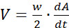
      where w denotes the width of the field and dA/dt is the time derivative of A(t), i.e., the expansion rate of the cell-covered area.
2. Cell motility map
   1. Execute a particle image velocimetry (PIV) algorithm to characterize cell motility, and extract the extent of local movement "optical flow" between image pairs, but not to identify individual cells.
      NOTE: Here, an initial window size of 50 µm is used, as described in detail by Zamir et al.³⁵ and Czirok et al.³⁶, with an initial window size of 50 µm. The PIV analysis yields a velocity field v(x,t) for each image frame t and location (within the image) x.
   2. Extract the average speed of cell motility from v(x,t) as a spatial average calculated over the cell occupied area, as determined in section 7.1.
3. Manual cell tracking
   NOTE: While the PIV analysis provides an automatic assessment of cell motility, to focus on the behavior of individual cells often requires manual tracking. While several tools provide this functionality, it is very helpful if the manually positioned markers can be modified after their initial placement, and if tracking can be performed both forward and backward in time.
   1. Perform cell tracking with a custom-developed python tool (http://github.com/donnagreta/cm_track), which also provides basic editor functions such as deleting trajectory segments.
      NOTE: This manual tracking tool yields the positions P(i,t) of cell i at time t in a text file, and invoked as
      cm_track.py -i images/ -o track.dat
      where the time-lapse images are in the folder images/ and the position data is collected in the file track.dat (Figure 4).

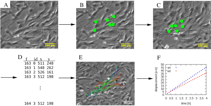
Figure 4: Analysis of individual cell trajectories. (A) Phase-contrast time-lapse micrographs are subjected to (B, C) a manual tracking procedure, which marks cells (green dots). (D) Cell positions (x,y) are stored for each cell distinguished by its ID and for each frame f. (E) Trajectories can be overlaid on the micrographs and color-coded to indicate temporal information. As an example, in each trajectory, a blue to red color palette indicates progressively later trajectory segments, with red and blue marking the initial and final cell locations, respectively. (F) Various statistical properties of trajectories, such as the mean square displacement, can be extracted and used to characterize the motility of various cell populations, which in this example include wildtype (wt, blue), and knockdown (kd, red) MEPM cells. The scalebars represent 100 µm. Please click here to view a larger version of this figure.

2. Overlay trajectories on images using a second tool, invoked as
   visdat.py -d track.dat -i images/ -o overlay/ -l999 -r3 -C2
3. Collect the images with the trajectories overlaid in the folder overlay.
   NOTE: In this example, cell position data are stored in the file track.dat, while the time-lapse image sequence is within the folder images. The rest of the parameters control the maximal length of the trajectories drawn (-l), the size of the symbols (-r), and the color scheme (-C) used.

4. Analysis of individual cell trajectories
   1. Characterize trajectories by the total path length
      ,
      and net displacement toward the wound
      ,
      where X denotes the projection of P in the direction perpendicular to the wound: the x coordinate of the positions when the wound is parallel to the y axis.
   2. Calculate the guidance efficiency as for each cell i and time point t³⁷. Characterize cultures by the population average of these single cell measures, evaluated at a suitable time point t.
5. Collective streaming motion of cells
   1. Characterize the local spatial correlations of cell movements by the average velocity of other cells that are in the vicinity of a moving cell, as described previously^38,39.
      NOTE: The computational code is available at https://github.com/aczirok/flowfield.
      1. Align a reference system with directions front, rear, left, and right to each vector v(x,t) (Figure 5A). Assign each of the surrounding cell or PIV velocity vector to the appropriate spatial cell of the reference system (Figure 5B). Repeat the procedure as each vector serves as the origin of the reference systems (Figure 5C,D) so that a given velocity vector is assigned to multiple bins.
         NOTE: A data point could be in front of a vector, and to the left of another one.
      2. Rotate the reference systems into a common orientation (Figure 5C,F) and pool them (Figure 5G).
         NOTE: The average of each bin of the pooled velocity data is a velocity vector (U) that is indicative of spatial correlation: the average is a measure of a shared velocity component (Figure 5H).
      3. Fit the U(x) flow fields with an exponential function , where a, x0 and U0 are fitting parameters. Out of the three fitting parameters, focus on x0, the correlation length (Figure 5I,J), which is the characteristic distance where local velocity-velocity correlations disappear.

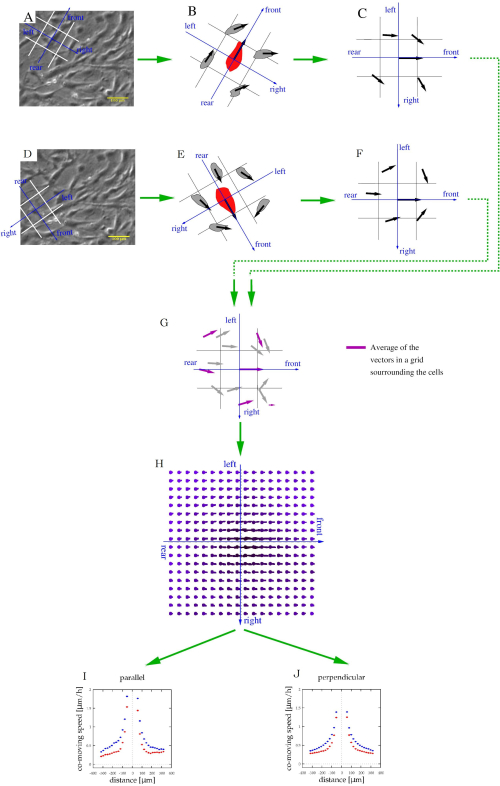
Figure 5: Characterization of stream formation of cultured cells. (A,D) Phase-contrast time-lapse images from Figure 4A are used to identify cell movements. For each moving cell, a frame of reference (blue) and spatial bins (white) were co-aligned to categorize adjacent cells as being in the front, rear, left, or right. (B,E) The velocity of adjacent cells (black vectors) was related to the same frame of reference (C,F). This procedure was repeated for each cell and time-point. (G) After pooling this local information, each bin will contain multiple velocity vectors (gray), which can be averaged to determine the average co-moving velocity (magenta arrows) at various locations relative to an average motile cell. (H) The average velocity map thus characterizes the typical cell velocities at various locations relative to a moving cell. (I,J) Finally, this field was sampled along the front-rear (parallel) axis and also along the left-right (perpendicular) axis. Please click here to view a larger version of this figure.

Results

The dissection of palatal shelves is illustrated in Figure 1. The sequence of incisions is designed to minimize slippage of the tissue. Following the removal of the head (Figure 1A,B), the lower jaw is removed (Figure 1B,C). The incision of the upper part of the head (Figure 1C,D) is done to stabilize the tissue when placed upside down (

Discussion

Palatal shelf elevation constitutes a vertical to horizontal remodeling event^1,3,4,9,11. It is postulated that this remodeling process requires palatal shelf mesenchymal cells to behave coordinately. The analyses with wildtype MEPM cells show that this cell behavior is intrinsic and can be quantitated²¹. Thus, these assays can be used t...

Materials

List of materials used in this article

Name	Company	Catalog Number	Comments
Beaker, 250 mL (x2)	Fisher Scientific	FB-100-250
CO2	Matheson Gas	UN1013
Conical tubes, 15 mL (x1)	Midwest Scientific	C15B
Debian operating system			computational analysis of time-lapse images
Dulbecco's Modified Eagles Medium/High Glucose with 4 mM L-Glutamine and Sodium Pyruvate	Cytiva Life Sciences	SH30243.01
EtOH, 100%	Decon Laboratories	2701
EVOS FL Auto	ThermoFisher Scientific	AMAFD1000
EVOS Onstage Incubator	ThermoFisher Scientific	AMC1000
EVOS Onstage Vessel Holder, Multi-Well Plates	ThermoFisher Scientific	AMEPVH028
Fetal Bovine Serum	Corning	35-010-CV
Fine point #5 Stainless Steel Forceps (x2)	Fine Science Tools	11295-10	Dissection
Instrument sterilizer bead bath	Fine Science Tools	18000-45
Microcetrifuge tubes, 1.5mL	Avant	2925
Micro-Dissecting Stainless Steel Scissors, Straight	Roboz	RS-5910	Dissection
NucBlue (Hoechst) Live Ready Probes	ThermoFisher Scientific	R37605
Penicillin Streptomycin Solution, 100x	Corning	30-002-CI
Silicone Insert, 2-well	Ibidi	80209
Small Perforated Stainless Steel Spoon	Fine Science Tools	MC17C	Dissection
Spring Scissors, 4 mm	Fine Science Tools	15018-10
Sterile 10 cm dishe(s)	Corning	430293
Sterile 12-well plate(s)	PR1MA	667512
Sterile 6-well plate(s)	Thermo Fisher Scientific	140675
Sterile PBS	Corning	21-031-CV
Sterile plastic bulb transfer pipette	ThermoFisher Scientific	202-1S
Trypsin, 0.25%	ThermoFisher Scientific	25200056

References

- Bush, J. O., Jiang, R. Palatogenesis: morphogenetic and molecular mechanisms of secondary palate development. Development. 139 (2), 231-243 (2012).
- Mossey, P. A., Little, J., Munger, R. G., Dixon, M. J., Shaw, W. C. Cleft lip and palate. Lancet. 374 (9703), 1773-1785 (2009).
- Lan, Y., Xu, J., Jiang, R. Cellular and molecular mechanisms of palatogenesis. Current Topics in Developmental Biology. 115, 59-84 (2015).
- Li, C., Lan, Y., Jiang, R. Molecular and cellular mechanisms of palate development. Journal of Dental Research. 96 (11), 1184-1191 (2017).
- Gritli-Linde, A. The etiopathogenesis of cleft lip and cleft palate: usefulness and caveats of mouse models. Current Topics in Developmental Biology. 84, 37(2008).
- Meng, L., Bian, Z., Torensma, R., Vonden Hoff, J. W. Biological mechanisms in palatogenesis and cleft palate. Journal of Dental Research. 88 (1), 22-33 (2009).
- Dixon, M. J., Marazita, M. L., Beaty, T. H., Murray, J. C. Cleft lip and palate: understanding genetic and environmental influences. Nature Reviews Genetics. 12 (3), 167-178 (2011).
- Kousa, Y. A., Schutte, B. C. Toward an orofacial gene regulatory network. Developmental Dynamics. 245 (3), 220-232 (2016).
- Jin, J. Z., et al. Mesenchymal cell remodeling during mouse secondary palate reorientation. Developmental Dynamics. 239 (7), 2110-2117 (2010).
- Yu, K., Ornitz, D. M. Histomorphological study of palatal shelf elevation during murine secondary palate formation. Developmental Dynamics. 240 (7), 1737-1744 (2011).
- Chiquet, M., Blumer, S., Angelini, M., Mitsiadis, T. A., Katsaros, C. Mesenchymal remodeling during palatal shelf elevation revealed by extracellular matrix and F-actin expression patterns. Frontiers in Physiology. 7, 392(2016).
- Paul, B. J., et al. ARHGAP29 mutation is associated with abnormal oral epithelial adhesions. Journal of Dental Research. 96 (11), 1298-1305 (2017).
- Hall, E. G., et al. SPECC1L regulates palate development downstream of IRF6. Human Molecular Genetics. 29 (5), 845-858 (2020).
- Walker, B. E., Fraser, F. C. Closure of the secondary palate in three strains of mice. Journal of Embryology and Experimental Morphology. 4 (2), 176-189 (1956).
- Jin, J. Z., Li, Q., Higashi, Y., Darling, D. S., Ding, J. Analysis of Zfhx1a mutant mice reveals palatal shelf contact-independent medial edge epithelial differentiation during palate fusion. Cell Tissue Research. 333 (1), 29-38 (2008).
- Kouskoura, T., et al. The etiology of cleft palate formation in BMP7-deficient mice. PLoS One. 8 (3), 59463(2013).
- Lan, Y., Zhang, N., Liu, H., Xu, J., Jiang, R. Golgb1 regulates protein glycosylation and is crucial for mammalian palate development. Development. 143 (13), 2344-2355 (2016).
- He, F., et al. Wnt5a regulates directional cell migration and cell proliferation via Ror2-mediated noncanonical pathway in mammalian palate development. Development. 135 (23), 3871-3879 (2008).
- Lan, Y., Qin, C., Jiang, R. Requirement of hyaluronan synthase-2 in craniofacial and palate development. Journal of Dental Research. 98 (12), 1367-1375 (2019).
- Yonemitsu, M. A., Lin, T. Y., Yu, K. Hyaluronic acid is required for palatal shelf movement and its interaction with the tongue during palatal shelf elevation. Developmental Biology. 457 (1), 57-68 (2020).
- Goering, J. P., et al. SPECC1L-deficient palate mesenchyme cells show speed and directionality defect. Scientific Reports. 11 (1), 1452(2021).
- Fantauzzo, K. A., Soriano, P. PI3K-mediated PDGFRalpha signaling regulates survival and proliferation in skeletal development through p53-dependent intracellular pathways. Genes and Development. 28 (9), 1005-1017 (2014).
- Vasudevan, H. N., Soriano, P. SRF regulates craniofacial development through selective recruitment of MRTF cofactors by PDGF signaling. Developmental Cell. 31 (3), 332-344 (2014).
- Vasudevan, H. N., Mazot, P., He, F., Soriano, P. Receptor tyrosine kinases modulate distinct transcriptional programs by differential usage of intracellular pathways. Elife. 4, 07186(2015).
- Gao, L., et al. 2,3,7,8-Tetrachlorodibenzo-p-dioxin and TGFbeta3-mediated mouse embryonic palatal mesenchymal cells. Dose Response. 17 (1), 1559325818786822(2019).
- Iyyanar, P. P. R., Nazarali, A. J. Hoxa2 inhibits bone morphogenetic protein signaling during osteogenic differentiation of the palatal mesenchyme. Frontiers in Physiology. 8, 929(2017).
- Jiang, Z., Pan, L., Chen, X., Chen, Z., Xu, D. Wnt6 influences the viability of mouse embryonic palatal mesenchymal cells via the beta-catenin pathway. Experimental and Therapeutic Medicine. 14 (6), 5339-5344 (2017).
- Liu, X., et al. Negative interplay of retinoic acid and TGF-beta signaling mediated by TG-interacting factor to modulate mouse embryonic palate mesenchymal-cell proliferation. Birth Defects Research Part B: Developmental and Reproductive Toxicology. 101 (6), 403-409 (2014).
- Bush, J. O., Soriano, P. Ephrin-B1 forward signaling regulates craniofacial morphogenesis by controlling cell proliferation across Eph-ephrin boundaries. Genes & Development. 24 (18), 2068-2080 (2010).
- Mo, J., Long, R., Fantauzzo, K. A. Pdgfra and Pdgfrb genetically interact in the murine neural crest cell lineage to regulate migration and proliferation. Frontiers in Physiology. 11, 588901(2020).
- He, F., Soriano, P. A critical role for PDGFRalpha signaling in medial nasal process development. PLoS Genetics. 9 (9), 1003851(2013).
- Fantauzzo, K. A., Soriano, P. Generation of an immortalized mouse embryonic palatal mesenchyme cell line. PLoS One. 12 (6), 0179078(2017).
- Wu, K., Gauthier, D., Levine, M. D. Live cell image segmentation. IEEE Transactions on Biomedical Engineering. 42 (1), 1-12 (1995).
- Neufeld, Z., et al. The role of Allee effect in modelling post resection recurrence of glioblastoma. PLoS Computational Biology. 13 (11), 1005818(2017).
- Zamir, E. A., Czirok, A., Rongish, B. J., Little, C. D. A digital image-based method for computational tissue fate mapping during early avian morphogenesis. Annals of Biomedical Engineering. 33 (6), 854-865 (2005).
- Czirok, A., et al. Optical-flow based non-invasive analysis of cardiomyocyte contractility. Scientific Reports. 7 (1), 10404(2017).
- Biggs, L. C., et al. Interferon regulatory factor 6 regulates keratinocyte migration. Journal of Cell Science. 127, Pt 13 2840-2848 (2014).
- Czirok, A., Varga, K., Mehes, E., Szabo, A. Collective cell streams in epithelial monolayers depend on cell adhesion. New Journal of Physics. 15, 75006(2013).
- Szabo, A., et al. Collective cell motion in endothelial monolayers. Physical Biology. 7 (4), 046007(2010).
- Gulyas, M., Csiszer, M., Mehes, E., Czirok, A. Software tools for cell culture-related 3D printed structures. PLoS One. 13 (9), 0203203(2018).
- Soderholm, J., Heald, R. Scratch n' screen for inhibitors of cell migration. Chemistry & Biology. 12 (3), 263-265 (2005).
- Riahi, R., Yang, Y., Zhang, D. D., Wong, P. K. Advances in wound-healing assays for probing collective cell migration. Journal of Laboratory Automation. 17 (1), 59-65 (2012).
- Svensson, C. M., Medyukhina, A., Belyaev, I., Al-Zaben, N., Figge, M. T. Untangling cell tracks: Quantifying cell migration by time lapse image data analysis. Cytometry Part A. 93 (3), 357-370 (2018).
- Fantauzzo, K. A., Soriano, P. PDGFRbeta regulates craniofacial development through homodimers and functional heterodimers with PDGFRalpha. Genes & Development. 30 (21), 2443-2458 (2016).
- Rafi, S. K., et al. Anti-epileptic drug topiramate upregulates TGFβ1 and SOX9 expression in primary embryonic palatal mesenchyme cells: Implications for teratogenicity. PLoS ONE. , In Press (2021).
Access restricted. Please log in or start a trial to view this content.
Reprints and Permissions