The method of standard addition is a quantitative analysis technique used to minimize matrix effects that interfere with analyte measurement signals.
Unknown component concentrations are often elucidated through a range of analytical techniques, such as light spectroscopy, mass spectrometry, and electrochemistry. However, the measurement can be affected by other components in the sample, called the matrix, and cause the inadvertent reduction or enhancement of the signal, called matrix effects. These effects can skew results and cause significant errors in analysis.
The method of standard addition can be used to minimize matrix effects on measurement signals. This is performed by adding precise volumes of a known analyte solution to the sample.
This video will introduce the basics of the standards addition method, and demonstrate how to perform the technique in the laboratory using a fluorescence measurement.
Matrix effects can arise in complex samples where a number of other molecules interact with the analyte. For example, this can occur when molecules bind or agglomerate with the analyte, thereby changing its ability to fluoresce. Or the matrix may change the ionic strength of the overall solution, changing specific properties of the analyte.
To mitigate these effects using the method of standard addition, a range of volumes of an analyte standard solution is added to equal volumes of the sample. The solution volumes are then made equal using solvent.
Then, the signal is measured for the samples with and without the standard addition. The data are plotted as intensity versus the amount of the standard added to the sample, rather than a classic calibration curve. The actual concentration of the analyte in any given flask is defined by the following equation. The instrumental response will equal some constant times the concentration of analyte. The resulting equation takes the linear form y=mx+b. Thus, when the plot is extrapolated to zero absorbance, the intercept is equal to the unknown concentration of the sample.
The signal plot must be linear over the concentration range of concern. Also, the interference should not vary as the ratio of analyte to sample matrix changes. Finally, the matrix itself should not generate any measurement signals on its own.
The following experiment studies aluminum, a non-fluorescent species, by reacting it with 8-hydroxyquinoline, or 8HQ, to form the fluorescent ALQ3 complex.
The fluorescence of the aluminum complex in an organic solvent is measured, and then related to the concentration of the original aluminum solution. This approach is common in the analysis of metal ions.
Now that the basics of the method of standard addition have been outlined, and the basics of the experiment explained, let’s perform the technique in the laboratory.
First, prepare the 100-ppm aluminum stock solution in water, and then use it to prepare a 1-ppm standard solution.
Next, add 2 g of 8-hydroxyquinoline, or 8HQ, to a 100-mL volumetric flask.
Carefully add 5.74 mL glacial acetic acid, then dilute to the 100-mL mark with deionized water. This step enables the 8HQ to dissolve in the aqueous phase.
Next, prepare the buffer by adding 20 g of ammonium acetate and 7 mL of 30% ammonium hydroxide to a 100-mL marked bottle and dilute. Verify the pH with a pH indicator stick. This buffer helps neutralize the acid in the 8HQ solution when combined.
Other reagents needed include anhydrous sodium sulfate and spectrophotometric grade chloroform.
Now prepare the samples, in this case by extracting the aqueous sample into the organic phase using liquid-liquid extraction. Place six 125-mL separatory funnels onto ring-stand rings inside the hood. Make sure all glassware is scrupulously clean, as dirty glassware will skew results. Sequentially label the funnels “blank”, “0”, “1”, “2”, “3”, and “4”.
Using a pipette, add 25 mL of the unknown aluminum solution to each of the five separatory funnels labeled “0” through “4”. Prepare the blank by adding 25 mL of deionized water to the funnel labeled “blank”.
Next, add 1, 2, 3, and 4 mL of the 1-ppm standard solution to the corresponding numbered funnels. Add no standard solution to the blank or 0 funnels.
Add 1 mL of the 8HQ solution and 3 mL of buffer solution to each of the 6 funnels.
Perform a liquid-liquid extraction by adding 10 mL of chloroform to each flask. Shake the funnel vigorously, and occasionally vent the funnel to release pressure buildup. Place the funnel back into the ring, and allow the liquid layers to separate.
Next, collect the chloroform phase in a clean, dry, and labeled 100-mL beaker. Since chloroform has a higher density than water, it is the lower layer in the funnel.
Transfer the chloroform extract into a 25-mL volumetric flask, and cap each flask to prevent evaporation.
Perform a second liquid-liquid extraction on the remaining aqueous solution, by adding 10 mL of chloroform to each funnel. Shake the funnel, as before, to transfer any remaining analyte to the chloroform phase. There should be no yellow color left in the top aqueous phase.
Repeat the second extraction for each funnel, then collect the chloroform phases in corresponding labeled beakers. Pour the collected chloroform into their respective volumetric flasks, and dilute to the mark with fresh chloroform.
To remove trace water, add about 1 g of anhydrous sodium sulfate to each of the six 100-mL beakers. Transfer the solutions back into their respective beakers, and swirl to facilitate dehydration of the sample.
Decant the chloroform extract into a quartz fluorimeter cell.
Set up the fluorimeter according to the manufacturers instructions and set the voltage to 400 V. Next, open the data acquisition program on the computer.
Use sample 2 to determine the best excitation and emission wavelengths. Set the emission wavelength to 500 nm, and run an excitation scan from 335–435 nm, with a scan speed of 2 nm/s.
From the fluorescence plot, determine the maximum wavelength for excitation. Set the instrument to that excitation wavelength value, in this case 399 nm.
Next, determine the emission wavelength by performing a scan from 450–550 nm. From the resulting fluorescence plot, determine the maximum wavelength and set the emission wavelength, in this case 520 nm.
Measure each sample, including the blank at the selected excitation and emission wavelength. Record each fluorescence intensity reading.
Subtract the measured fluorescence of the blank sample from each of the other 5 samples.
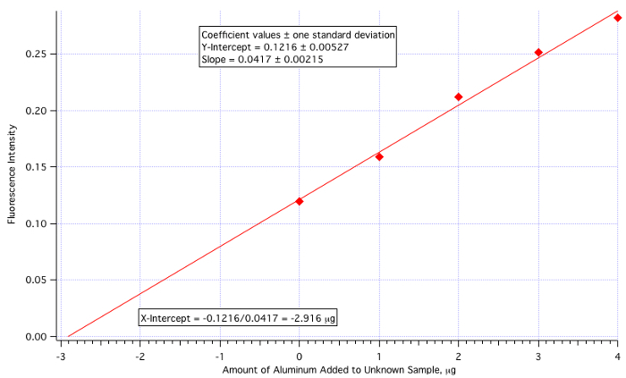
Plot the fluorescence intensity of each of the five samples versus the amount of aluminum added to the sample. Determine the least squares value of the resulting plot, and record the slope and intercept.
The plot of fluorescence intensity vs. amount of aluminum added yielded a least-square line as shown. The amount of aluminum in the sample can then be calculated using this line. Since the amount of unknown added was 25 mL, the determined value, 2.916 μg is divided by 25 mL. This gives a final result of 0.117 μg/mL, or 0.117 ppm. This is quite close to the known value of 0.110 ppm.
Now, let’s look at some other analytical techniques that can have skewed results due to matrix effects.
Atomic absorption spectroscopy is an analytical method that measures the absorbance of light by a target analyte in the gaseous phase. For most samples, a simple calibration curve relating absorption to sample concentration, can serve as a reliable method to quantify an unknown concentration.
However, this technique can lose accuracy if other components of the mixture interact with the target analyte and suppress or enhance absorption. The standard addition method can be used in this case to account for the effects of these interactions, especially in samples where the matrix cannot be removed prior to analysis.
Instrument calibration plays a crucial role in the accuracy of a measurement. The method of standard addition is often used to aid in calibration of instruments such as ICP-MS. ICP-MS is a comparative method, meaning that the measurement of an unknown sample is based on the measurement of a chemical standard.
Thus, the uncertainty of a measurement of an unknown can’t be better than the uncertainty of the calibration. The method of standard addition can therefore be used to create a calibration curve that is more accurate than the standard method, and accounts for matrix interactions in the sample.
Many biological molecules are analyzed using high-performance liquid chromatography, or HPLC. HPLC is a technique that separates and analyzes complex mixtures based on molecule properties such as polarity, charge, and size. The time at which the analyte leaves the column enables the user to identify each component in the mixture.
Biological molecules can often interact in a mixture, and are greatly affected by the matrix they are suspended in. Often, the method of standard addition is used to create a calibration curve that accounts for these affects.
You’ve just watched JoVE’s introduction to the method of standard addition. You should now understand how to perform the technique to account for matrix effects in sample analysis.
Thanks for watching!