JoVE Science Education
Mechanical Engineering
This content is Free Access.
JoVE Science Education Mechanical Engineering
Hydraulic Jumps
  • 00:07Overview
  • 01:05Principles of Hydraulic Jumps
  • 03:57Preparing the Experiment
  • 04:55Data Collection
  • 06:00Analysis and Results
  • 07:59Applications
  • 08:48Summary

Salti idraulici

English

Share

Overview

Fonte: Alexander S Rattner e Mahdi Nabil; Dipartimento di Ingegneria Meccanica e Nucleare, The Pennsylvania State University, University Park, PA

Quando il liquido scorre lungo un canale aperto ad alta velocità, il flusso può diventare instabile e lievi disturbi possono causare la transizione improvvisa della superficie superiore del liquido a un livello più alto (Fig. 1a). Questo forte aumento del livello del liquido è chiamato salto idraulico. L’aumento del livello del liquido provoca una riduzione della velocità media del flusso. Di conseguenza, l’energia cinetica del fluido potenzialmente distruttiva viene dissipata sotto disegno di calore. I salti idraulici sono appositamente progettati in grandi opere idriche, come gli sfioratori delle dighe, per prevenire danni e ridurre l’erosione che potrebbe essere causata da flussi in rapido movimento. I salti idraulici si verificano naturalmente anche in fiumi e torrenti e possono essere osservati in condizioni domestiche, come il deflusso radiale di acqua da un rubinetto su un lavandino (Fig. 1b).

In questo progetto, verrà costruita una struttura sperimentale a flusso a canale aperto. Verrà installata una chiusa, che è un cancello verticale che può essere sollevato o abbassato per controllare la velocità di scarico dell’acqua da un serbatoio a monte a uno sfioratore a valle. Verrà misurata la portata necessaria per produrre salti idraulici all’uscita del cancello. Questi risultati saranno confrontati con valori teorici basati su analisi di massa e quantità di moto.

Figure 1
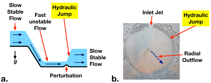
Figura 1: a. Salto idraulico che si verifica a valle di uno sfioratore a causa di una leggera perturbazione di un flusso instabile ad alta velocità. b. Esempio di salto idraulico nel deflusso radiale dell’acqua da un rubinetto domestico.

Principles

Nei flussi a canale aperto, il liquido è confinato solo da un limite solido inferiore e la sua superficie superiore è esposta all’atmosfera. Un’analisi del volume di controllo può essere eseguita su una sezione di un flusso a canale aperto per bilanciare il trasporto in ingresso e in uscita di massa e quantità di moto (Fig 2). Se le velocità sono assunte uniformi all’ingresso e all’uscita del volume di controllo(V1 e V2 rispettivamente) con le corrispondenti profondità del liquido H1 e H2, allora un bilancio del flusso di massa costante si riduce a:

Equation 1 (1)

L’analisi del momento in direzione xdi questo volume di controllo bilancia le forze della pressione idrostatica (dovuta alla profondità del fluido) con le portate del momento in ingresso e in uscita (Eqn. 2). Le forze di pressione agiscono verso l’interno sui due lati del volume di controllo, e sono uguali al peso specifico del liquido (densità del liquido volte accelerazione gravitazionale: ρg), moltiplicato per la profondità media del liquido su ciascun lato (H1/2, H2/2), moltiplicata l’altezza su cui la pressione agisce su ciascun lato (H1, H2). Ciò si traduce nell’espressione quadratica sul lato sinistro di Eqn. 2. Le portate di quantità di moto attraverso ciascun lato (Eqn. 2, lato destro) sono uguali alle portate di massa del liquido attraverso il volume di controllo (in: Equation 2 , out: Equation 3 ) moltiplicato per le velocità del fluido (V1, V2).

Equation 4 (2)

Eqn. 1 può essere sostituito in Eqn. 2 per eliminare V2. Il numero di Froude ( Equation 5 ) può anche essere sostituito in, che rappresenta la forza relativa del momento del fluido di afflusso alle forze idrostatiche. L’espressione risultante può essere indicata come:

Equation 6 (3)

Questa equazione cubica ha tre soluzioni. Uno è H1 = H2, che dà il normale comportamento del canale aperto (profondità di ingresso = profondità di uscita). Una seconda soluzione dà un livello di liquido negativo, che non è fisico e può essere eliminato. La soluzione rimanente consente un aumento della profondità (salto idraulico) o una diminuzione della profondità (depressione idraulica), a seconda del numero di Froude in ingresso. Se il numero di Froude in ingresso (Fr1) è maggiore di uno, il flusso è chiamato supercritico (instabile) e ha un’elevata energia meccanica (energia potenziale cinetica + gravitazionale). In questo caso, un salto idraulico può formarsi spontaneamente o a causa di qualche disturbo al flusso. Il salto idraulico dissipa l’energia meccanica in calore, riducendo significativamente l’energia cinetica e aumentando leggermente l’energia potenziale del flusso. L’altezza di uscita risultante è data da Eqn. 4 (una soluzione a Eqn. 3). Una depressione idraulica non può verificarsi se Fr1 > 1 perché aumenterebbe l’energia meccanica del flusso, violando la seconda legge della termodinamica.

Equation 7 (4)

La forza dei salti idraulici aumenta con i numeri di Froude in ingresso. All’aumentare di Fr1, la grandezza di H2/ H1 aumenta e una porzione maggiore di energia cinetica in ingresso viene dissipata come calore [1].

Figure 2
Figura 2: Volume di controllo di una sezione di un flusso a canale aperto contenente un salto idraulico. Sono indicate le portate di massa e di quantità di massa e di quantità di moto in ingresso e in uscita per unità di larghezza. Forze idrostatiche per unità di larghezza indicate nel diagramma inferiore.

Procedure

NOTA: questo esperimento utilizza una pompa sommergibile relativamente potente. La pompa deve essere collegata solo a una presa GFCI per ridurre al minimo i rischi elettrici. Assicurarsi che nessun altro dispositivo alimentato a corrente condizionata sia in funzione vicino all’esperimento. 1. Fabbricazione dell’impianto di flusso a canale aperto e del serbatoio (vedi diagramma e fotografia, Fig. 3) Lunghezze di taglio di ~ 6,0 mm di spessore × foglio acrilico trasparente largo 9,5 cm con le seguenti lunghezze: 2×15 cm, 2×25 cm, 1×34 cm, 1×41 cm (Fig. 3a). Si consiglia di utilizzare una sega da tavolo o una fresa laser per garantire che i bordi siano relativamente piatti e che i fogli abbiano lo stesso spessore. Tagliare fori negli angoli in basso a destra dei due fogli acrilici da 60 × 45 cm per montare il flussometro (Fig. 3a). Tagliare un foro nella parte superiore destra del foglio frontale per installare la valvola di controllo del flusso. Utilizzare cemento acrilico(ad esempio,SCIGRIP 16) per incollare i pannelli acrilici come indicato in Fig. 3a. Garantire un’adeguata ventilazione e indossare guanti quando si maneggia il cemento acrilico. È utile applicare il cemento con una siringa ad ago e utilizzare del nastro adesivo per posizionare i pannelli durante la polimerizzazione. Lasciare polimerizzare il cemento per 24 – 48 ore. Installare il flussometro sul pannello frontale e fissare con le viti fornite. Installare 1 raccordi riducenti da NPT a 1/2 NPT sulle porte di ingresso e uscita del flussometro. Installare adattatori per raccordi spinati da 1/2 NPT a 0,5 pollici di diametro interno a tali raccordi. Installare un 0.5 in. ID e un 0.75 in. Raccordo spinato ID sulla valvola a saracinesca (controllo della portata). Collegare il raccordo spinato alla pompa sommergibile con un tubo di lunghezza di circa 20 cm in modo che la maniglia della valvola si alllinei con il foro in alto a destra dell’involucro acrilico (Fig. 3b-c). Inserire la pompa nel serbatoio inferiore e installare la valvola in modo che lo stelo della valvola passi attraverso il foro di montaggio e la maniglia sia all’esterno dell’involucro (Fig. 3c). Inserire un pannello acrilico verticale vicino alla porzione di ingresso dell’impianto di flusso in modo che vi sia un’apertura di circa 5,0 mm sotto di esso (Fig. 3b-c). Questo componente fungerà da paratoiae può essere sollevato e abbassato per controllare il flusso dal serbatoio superiore al canale. Riempire liberamente il serbatoio superiore con un tampone abrasivo in lana di acciaio inossidabile. Questo aiuta a distribuire uniformemente il flusso dell’acqua in ingresso attraverso il canale. Collegare l’uscita della valvola all’ingresso del flussometro con una lunghezza di tubo di plastica morbida. Collegare l’uscita del flussometro al serbatoio superiore con tubi di plastica. Assicurarsi che l’ingresso del tubo al serbatoio superiore sia ben ancorato in modo che non oscilli quando la pompa è accesa. Riempire il serbatoio inferiore con acqua. 2. Esecuzione dell’esperimento Misurare l’altezza dello spazio sotto il cancello utilizzando un righello e indicare il valore come H1. Accendere la pompa e regolare la portata utilizzando la valvola a varie portate (5 – 15 l min-1). Utilizzare un righello per misurare la profondità del liquido a valle del cancello (H2) per ciascun caso. Osservare qualitativamente le forme dei salti idraulici che si formano a diverse portate. Guarda la portata minima di soglia per la formazione di un salto idraulico. Più nitidi, maggiore ampiezza (H2 -H1), i salti dovrebbero verificarsi a portate più elevate. 3. Analisi dei dati Per ogni caso di portata, calcolare la velocità di ingresso, V1, dalla portata volumetrica. dove è la portata volumetrica e W è la larghezza del canale. Valutare il numero di Froude in ingresso ( ) e la profondità teorica del liquido a valle per ciascun caso (Eqn. 4). Confronta questi valori con le profondità di salto a valle misurate. Figura 3: a. Schema e dimensioni della struttura dell’impianto.b. Diagramma di flusso dell’impianto di salto idraulico.c. Fotografia etichettata dell’impianto sperimentale.

Results

Upstream Froude numbers (Fr1) and measured and theoretical downstream depths are summarized in Table 1. The measured threshold inlet flow rate for formation of a hydraulic jump corresponds to Fr1 = 0.9 ± 0.3, which matches the theoretical value of 1. At supercritical flow rates (Fr1 > 1) predicted downstream depths match theoretical values (Eqn. 4) within experimental uncertainty.

Table 1 – Measured upstream Froude numbers (Fr1) and downstream liquid depths for H1 = 5 ± 1 mm

Liquid Flow Rate

(Equation 9, l min-1)

Upstream Froude Number (Fr1) Measured Downstream Depth (H2) Predicted Downstream Depth (H2) Notes
6.0   ± 0.5 0.9 ± 0.3 5 ± 1 5 ± 1 Threshold Froude number for hydraulic jump
11.0 ± 0.5 1.7 ± 0.5 11 ± 1 10 ± 2
12.0 ± 0.5 1.9 ± 0.6 12 ± 1 11 ± 2
13.5 ± 0.5 2.1 ± 0.6 14 ± 1 13 ± 2

Photographs of the hydraulic jumps from the above cases are presented in Fig. 4. No jump is observed for Equation 9 = 6.0 l min-1 (Fr1 = 0.9). Jumps are observed for the two other cases with Fr1 > 1. A stronger, higher amplitude, jump is observed at the higher flow rate supercritical case.

Figure 4
Figure 4: Photograph of hydraulic jumps, showing critical condition (no jump, Fr1 = 0.9) and jumps at Fr1 = 1.9, 2.1.

Applications and Summary

This experiment demonstrated the phenomena of hydraulic jumps that form at supercritical conditions (Fr > 1) in open channel flows. An experimental facility was constructed to observe hydraulic jump phenomena at varying flow rates. Downstream liquid depths were measured and matched with theoretical predictions.

In this experiment, the maximum reported inlet Froude number was 2.1. The pump was rated to deliver significantly higher flow rates, but resistance in the flow meter limited measurable flow rates to ~14 l min-1. In future experiments, a pump with a greater head rating or a lower pressure drop flow meter may enable a broader range of studied conditions.

Hydraulic jumps are often engineered into hydraulic systems to dissipate fluid mechanical energy into heat. This reduces the potential for damage by high velocity liquid jetting from spillways. At high channel flow velocities, sediment can be lifted up from streambeds and fluidized. By reducing flow velocities, hydraulic jumps also reduce the potential for erosion and scouring around pilings. In water treatment plants, hydraulic jumps are sometimes used to induce mixing and aerate flow. The mixing performance and gas entrainment from hydraulic jumps can be observed qualitatively in this experiment.

For all of these applications, momentum analyses across hydraulic jumps, as discussed here, are key tools for predicting hydraulic system behavior. Similarly, scale model experiments such as those demonstrated in this project, can guide the design of open-channel flow geometries and hydraulic equipment for large-scale engineering applications.

References

  1. Cimbala, Y.A. Cengel, Fluid Mechanics Fundamentals and Applications, 3rd edition, McGraw-Hill, New York, NY, 2014.

Transcript

A hydraulic jump is a phenomenon that occurs in fast-moving open flows when the flow becomes unstable. When a jump occurs, the height of the liquid surface increases abruptly resulting in an increased depth and decreased average flow velocity downstream. An important side effect of this phenomenon is that much of the kinetic energy in the upstream flow is dissipated as heat. Although hydraulic jumps often arise naturally, such as in rivers or the flow into a household sink, they are also purposely engineered into large waterworks to minimize erosion, or increase mixing. This video will illustrate the principles behind hydraulic jumps in a straight channel and then demonstrate the phenomenon experimentally using a small-scale open channel flow facility. After analyzing the results, some applications of hydraulic jumps will be discussed.

Consider the flow in a wide, straight section of an open channel where a hydraulic jump occurs and construct a control volume on a sluice around the jump. If the flow velocity is uniform at the inlet and outlet, conservation of mass yields a simple relation between upstream and downstream fluid depths. Depth multiplied by velocity is constant. A second relation can be found by considering conservation of momentum. Mass transported across the input and output carries momentum with it equal to the corresponding mass flux multiplied by the flow velocity. Hydrostatic forces on the surface of the control volume also contribute to the momentum balance and must be included. These forces are equal to the average pressure on the surface multiplied by the area. At this point, it is useful to introduce the Froude number, a dimensionless quantity named after the English engineer and hydrodynamicist, William Froude. The Froude number characterizes the relative strength of fluid momentum to hydrostatic forces. Now, if the momentum relation is rewritten in terms of the Froude number, with the output velocity eliminated by substitution using the mass relation, the result is a cubic equation in terms of the ratio of downstream and upstream depths. This equation can be simplified by factoring out the trivial solution where the upstream and downstream depths are equal. The two remaining solutions are easily found using the quadratic equation, but the negative solution can be eliminated since it is non-physical. The remaining solution corresponds to an increase in depth, a hydraulic jump, or a decrease in depth, a hydraulic depression, based on the value of the upstream Froude number. If the upstream Froude number is greater than one, the flow has a high mechanical energy and is supercritical or unstable. A hydraulic depression cannot form in this regime because it would increase mechanical energy and violate the second law of thermodynamics. On the other hand, a hydraulic jump can form, either spontaneously or due to some disturbance in the flow. An input Froude number of one represents the minimum threshold for the onset of a hydraulic jump. Hydraulic jumps dissipate mechanical energy into heat, and significantly reduce the kinetic energy, while slightly increasing the potential energy of the flow. As the Froude number increases, so does the ratio of downstream to upstream depths and the amount of kinetic energy dissipated as heat. Now that we understand the principles behind hydraulic jumps, let’s examine them experimentally.

First, fabricate the open channel flow facility as described in the text. The facility has an upper and lower reservoir connected by an open channel. Water pumped from the lower reservoir is deposited in the upper reservoir with the flow rate controlled and measured by a valve and flow meter in line with the pump. Steel wool in the upper reservoir helps to evenly distribute the water across the width of the section, and the adjustable sluice gate controls the fluid depth as it enters the channel. After flowing through the channel, the fluid is deposited back into the lower reservoir. When the flow facility is assembled, set it up on a bench and remove any nearby electronic devices. Plug the pump into a GFCI outlet to minimize the risk of electrical shock, and then fill the lower reservoir with water. You are now ready to perform the experiment.

Adjust the sluice gate to approximately five millimeters. Measure the final height of the gap underneath the sluice gate using a ruler, and record this distance as the upstream flow depth, H1. When you are finished, turn on the pump and use the valve to maximize the flow rate without exceeding the scale on the flow meter. Use the ruler again to measure the fluid depth after the hydraulic jump. Record the flow rate, along with this second distance which is the downstream flow depth, H2. Before continuing, observe the shape of the hydraulic jump. You should notice larger, more abrupt transitions for higher flow rates, and smaller, more gradual transitions for lower flow rates. Now, repeat your measurements and observations for successively lower flow rates. Try to determine the minimum threshold flow rate for the formation of a hydraulic jump. Once you have found the threshold flow rate, you are ready to analyze the results.

For each volumetric flow rate, you should have a measurement of the downstream fluid depth. The upstream depth is the same for all cases. Complete the following calculations for each measurement and propagate uncertainties along the way. First, determine the inlet flow velocity. Divide the volumetric flow rate by the channel width and upstream depth. Next, evaluate the upstream Froude number using the definition given before, and substituting in the acceleration due to gravity, as well as the upstream height and velocity. Now, use the Froude number and the non-trivial solution for the jump height to calculate the theoretical downstream depth. Compare the theoretical prediction with the measured downstream depth. At supercritical flow rates, the predictions match the measured depths within experimental uncertainty. Look at your results for the threshold flow rate. Within experimental uncertainty, the Froude number is one, as we anticipated from the theoretical analysis. The rate of mechanical energy loss through the hydraulic jump can also be calculated from these data. First, calculate the mechanical energy of the fluid flowing into the jump, which is the sum of kinetic and potential energy flow rates at the inlet. Now, determine the output energy rate in the same way, but with values at the outlet. The rate of mechanical energy dissipation to heat is the difference between the input and output rates. In this experiment, the energy loss rate can reach about 40% of the inlet energy, or higher. These results highlight the effectiveness of momentum analyses and scale model experiments for understanding and predicting the behavior of hydraulic systems. Now let’s look at some other ways hydraulic jumps are utilized.

Hydraulic jumps are an important natural phenomenon with many engineering applications. Hydraulic jumps are often engineered into hydraulic systems to dissipate fluid mechanical energy into heat. This reduces the potential for damage by high velocity liquid jetting from spillways. At high channel flow velocities, sediment can be lifted up from streambeds and fluidized. By reducing flow velocities, hydraulic jumps also reduce the potential for erosion and scouring around pilings. In water treatment plants, hydraulic jumps are sometimes used to induce mixing and aerate flow. The mixing performance and gas entrainment from hydraulic jumps can be observed qualitatively in this experiment.

You’ve just watched JoVE’s introduction to hydraulic jumps. You should now understand how to use a control volume approach to predict the flow behavior, and how to measure this behavior using an open channel flow facility. You’ve also seen some practical uses for engineering hydraulic jumps in real applications. Thanks for watching.

Tags

Cite This
JoVE Science Education Database. JoVE Science Education. Hydraulic Jumps. JoVE, Cambridge, MA, (2023).