Hydraulic Jumps - JoVE Wordpress Development

JoVE Science Education
Mechanical Engineering

This content is Free Access.

JoVE Science Education Mechanical Engineering

Hydraulic Jumps

00:07Overview
01:05Principles of Hydraulic Jumps
03:57Preparing the Experiment
04:55Data Collection
06:00Analysis and Results
07:59Applications
08:48Summary

English العربية 中文 Nederlands Français Deutsch עברית Italiano 日本語 한국어 Português русский Español Türkçe

Saltos Hidráulicos

English

Overview

Fonte: Alexander S Rattner e Mahdi Nabil; Departamento de Engenharia Mecânica e Nuclear, Universidade Estadual da Pensilvânia, Parque Universitário, PA

Quando o líquido flui ao longo de um canal aberto em alta velocidade, o fluxo pode se tornar instável, e pequenas perturbações podem fazer com que a superfície superior líquida transite abruptamente para um nível mais alto (Fig. 1a). Este aumento acentuado no nível líquido é chamado de salto hidráulico. O aumento do nível líquido provoca uma redução na velocidade média de fluxo. Como resultado, a energia cinética potencialmente destrutiva do fluido é dissipada como calor. Os saltos hidráulicos são propositalmente projetados em grandes obras de água, como vertedouros de barragens, para evitar danos e reduzir a erosão que poderia ser causada por fluxos em movimento rápido. Saltos hidráulicos também ocorrem naturalmente em rios e córregos, podendo ser observados em condições domésticas, como o fluxo radial de água de uma torneira para uma pia (Fig. 1b).

Neste projeto, será construída uma instalação experimental de fluxo de canal aberto. Um portão de sluice será instalado, que é um portão vertical que pode ser levantado ou abaixado para controlar a taxa de descarga de água de um reservatório a montante para um vertedouro a jusante. A vazão necessária para produzir saltos hidráulicos na saída do portão será medida. Esses achados serão comparados com valores teóricos baseados em análises de massa e momento.

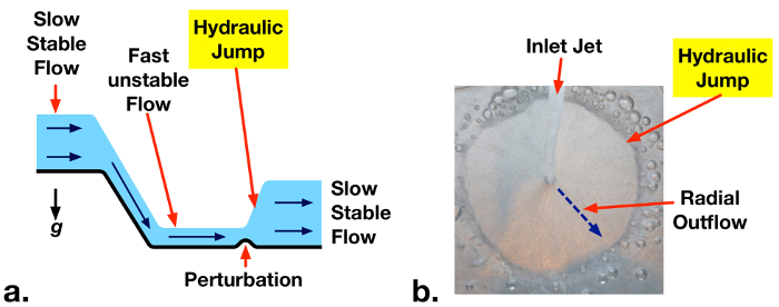
Figura 1: a. Salto hidráulico ocorrendo rio abaixo de um vertedouro devido a uma leve perturbação a um fluxo instável de alta velocidade. b. Exemplo de salto hidráulico no fluxo radial de água de uma torneira doméstica.

Principles

Em fluxos de canais abertos, o líquido é confinado apenas por um limite sólido inferior e sua superfície superior é exposta à atmosfera. Uma análise de volume de controle pode ser realizada em uma seção de fluxo de canal aberto para equilibrar o transporte de entrada e saída de massa e momento (Fig 2). Se as velocidades forem assumidas uniformes na entrada e saída do volume de controle(V₁ e V_{2, respectivamente)}com as profundidades líquidas correspondentes H₁ e H_2,então um equilíbrio constante de fluxo de massa reduz a:

(1)

A análise de impulso x-direção deste volume de controle equilibra forças da pressão hidrostática (devido à profundidade do fluido) com as taxas de fluxo de impulso de entrada e saída (Eqn. 2). As forças de pressão atuam para dentro nos dois lados do volume de controle, e são iguais à gravidade específica do líquido (densidade líquida vezes aceleração gravitacional: ρg), multiplicada pela profundidade líquida média de cada lado (H_1/2, H₂/2), multiplicada a altura sobre a qual a pressão age em cada lado (H₁, H₂). Isso resulta na expressão quadrática no lado esquerdo do Eqn. 2. As taxas de fluxo de impulso através de cada lado (Eqn. 2, lado direito) são iguais às taxas de fluxo de massa de líquido através do volume de controle (em: , out: ) multiplicadas pelas velocidades fluidas(V₁, V₂).

(2)

Eqn. 1 pode ser substituído em Eqn. 2 para eliminar V₂. O número de Froude também pode ser substituído, o que representa a força relativa do impulso fluido de entrada para forças hidrostáticas. A expressão resultante pode ser indicada como:

(3)

Esta equação cúbica tem três soluções. Um deles é H1 = H2, que dá o comportamento normal de canal aberto (profundidade de entrada = profundidade de saída). Uma segunda solução dá um nível líquido negativo, que não é físico, e pode ser eliminado. A solução restante permite um aumento de profundidade (salto hidráulico) ou uma diminuição da profundidade (depressão hidráulica), dependendo do número de froude de entrada. Se o número de Froude de entrada (Fr₁) for maior que um, o fluxo é chamado de supercrítico (instável) e tem alta energia mecânica (energia potencial cinética + gravitacional). Neste caso, um salto hidráulico pode se formar espontaneamente ou devido a alguma perturbação ao fluxo. O salto hidráulico dissipa a energia mecânica em calor, reduzindo significativamente a energia cinética e aumentando ligeiramente a energia potencial do fluxo. A altura de saída resultante é dada por Eqn. 4 (uma solução para Eqn. 3). Uma depressão hidráulica não pode ocorrer se o Padre₁ > 1 porque aumentaria a energia mecânica do fluxo, violando a segunda lei da termodinâmica.

(4)

A força dos saltos hidráulicos aumenta com os números de entrada froude. À medida que o Fr₁ aumenta, a magnitude de H₂/H₁ aumenta e uma porção maior de energia cinética de entrada é dissipada como calor [1].

Figura 2: Controle o volume de uma seção de um fluxo de canal aberto contendo um salto hidráulico. As taxas de fluxo de massa e de impulso por unidade são indicadas. Forças hidrostáticas por largura de unidade indicada em diagrama inferior.

Procedure

NOTA: Este experimento usa uma bomba submersível relativamente poderosa. A bomba só deve ser conectada a uma tomada GFCI para minimizar os riscos elétricos. Certifique-se de que nenhum outro dispositivo alimentado a/C esteja operando perto do experimento. 1. Fabricação de instalações de fluxo de canais abertos e tanque (ver diagrama e fotografia, Fig. 3) Corte de comprimentos de ~6,0 mm de espessura × folha de acrílico claro de 9,5 cm de largura com os seguintes comprimentos: 2×15 cm, 2×25 cm, 1×34 cm, 1×41 cm (Fig. 3a). Recomenda-se usar uma serra de mesa ou cortador a laser para garantir que as bordas sejam relativamente planas e que as folhas tenham espessura igual. Corte furos nos cantos inferiores direito das duas folhas acrílicas de 60 × de 45 cm para montar o medidor de fluxo (Fig. 3a). Corte um orifício no lado superior direito da folha frontal para instalar a válvula de controle de fluxo. Use cimento acrílico (por exemplo,SCIGRIP 16) para ligar os painéis acrílicos conforme indicado na Fig. 3a. Certifique-se de ventilação adequada e use luvas ao manusear o cimento acrílico. É útil aplicar cimento com uma seringa de agulha e usar fita adesiva para posicionar painéis durante a cura. Deixe o cimento curar por 24 a 48 horas. Instale o medidor de fluxo no painel frontal e afixe com os parafusos fornecidos. Instale 1 NPT a 1/2 NPT reduzindo os encaixes nas portas de entrada e saída do medidor de fluxo. Instale 1/2 NPT a 0,5 in. adaptadores de encaixe farpados de diâmetro interno nesses encaixes. Instale um 0,5 dentro. ID e 0,75 de dólar. Encaixe de farpado de ID na válvula do portão (controle da taxa de fluxo). Conecte o encaixe farpado à bomba submersível com um comprimento de tubo de ~20 cm para que a alça da válvula se a linha com o orifício no canto superior direito do gabinete acrílico (Fig. 3b-c). Insira a bomba no reservatório inferior e instale a válvula para que a haste da válvula passe pelo orifício de montagem e a alça esteja fora do compartimento (Fig. 3c). Insira um painel de acrílico vertical perto da porção de entrada da instalação de fluxo para que haja aproximadamente uma abertura de 5,0 mm abaixo dele (Fig. 3b-c). Este componente funcionará como o portão de esguicagem,podendo ser elevado e abaixado para controlar o fluxo do reservatório superior para o canal. Encha o reservatório superior livremente com uma almofada de limpeza de lã de aço inoxidável. Isso ajuda a distribuir o fluxo de água de entrada uniformemente através do canal. Conecte a saída da válvula à entrada do medidor de fluxo com um comprimento de tubo plástico macio. Conecte a saída do medidor de fluxo ao reservatório superior com tubos plásticos. Certifique-se de que a entrada do tubo para o reservatório superior esteja bem ancorada para que não se escora quando a bomba estiver ligada. Encha o reservatório inferior com água. 2. Realizar experimentos Meça a altura da abertura sob o portão usando uma régua e denote o valor como H1. Ligue a bomba e ajuste a taxa de fluxo usando a válvula para várias taxas de fluxo (5 – 15 l min-1). Use uma régua para medir a profundidade líquida rio abaixo do portão(H2) para cada caso. Observe qualitativamente as formas dos saltos hidráulicos que se formam em diferentes taxas de fluxo. Observe a taxa mínima de fluxo de limiar para a formação de um salto hidráulico. Maior amplitude mais acentuada(H2 -H1),os saltos devem ocorrer em taxas de fluxo mais altas. 3. Análise de dados Para cada estojo de vazão, calcule a velocidade de entrada, V1, a partir da taxa de fluxo volumoso. onde está a taxa de fluxo de volume e W é a largura do canal. Avalie o número de entrada Froude ( ) e a profundidade líquida a jusante teórica para cada caso (Eqn. 4). Compare esses valores com as profundidades de salto a jusante medidas. Figura 3: a. Esquema e dimensões da estrutura da instalação.b. Diagrama de fluxo da instalação de salto hidráulico.c. Fotografia rotulada de instalação experimental.

Results

Upstream Froude numbers (Fr₁) and measured and theoretical downstream depths are summarized in Table 1. The measured threshold inlet flow rate for formation of a hydraulic jump corresponds to Fr₁ = 0.9 ± 0.3, which matches the theoretical value of 1. At supercritical flow rates (Fr₁ > 1) predicted downstream depths match theoretical values (Eqn. 4) within experimental uncertainty.

Table 1 – Measured upstream Froude numbers (Fr₁) and downstream liquid depths for H₁ = 5 ± 1 mm

Liquid Flow Rate (, l min^-1)	Upstream Froude Number (Fr₁)	Measured Downstream Depth (H₂)	Predicted Downstream Depth (H₂)	Notes
6.0 ± 0.5	0.9 ± 0.3	5 ± 1	5 ± 1	Threshold Froude number for hydraulic jump
11.0 ± 0.5	1.7 ± 0.5	11 ± 1	10 ± 2
12.0 ± 0.5	1.9 ± 0.6	12 ± 1	11 ± 2
13.5 ± 0.5	2.1 ± 0.6	14 ± 1	13 ± 2

Photographs of the hydraulic jumps from the above cases are presented in Fig. 4. No jump is observed for = 6.0 l min^-1 (Fr₁ = 0.9). Jumps are observed for the two other cases with Fr₁ > 1. A stronger, higher amplitude, jump is observed at the higher flow rate supercritical case.

Figure 4: Photograph of hydraulic jumps, showing critical condition (no jump, Fr₁ = 0.9) and jumps at Fr₁ = 1.9, 2.1.

Applications and Summary

This experiment demonstrated the phenomena of hydraulic jumps that form at supercritical conditions (Fr > 1) in open channel flows. An experimental facility was constructed to observe hydraulic jump phenomena at varying flow rates. Downstream liquid depths were measured and matched with theoretical predictions.

In this experiment, the maximum reported inlet Froude number was 2.1. The pump was rated to deliver significantly higher flow rates, but resistance in the flow meter limited measurable flow rates to ~14 l min^-1. In future experiments, a pump with a greater head rating or a lower pressure drop flow meter may enable a broader range of studied conditions.

Hydraulic jumps are often engineered into hydraulic systems to dissipate fluid mechanical energy into heat. This reduces the potential for damage by high velocity liquid jetting from spillways. At high channel flow velocities, sediment can be lifted up from streambeds and fluidized. By reducing flow velocities, hydraulic jumps also reduce the potential for erosion and scouring around pilings. In water treatment plants, hydraulic jumps are sometimes used to induce mixing and aerate flow. The mixing performance and gas entrainment from hydraulic jumps can be observed qualitatively in this experiment.

For all of these applications, momentum analyses across hydraulic jumps, as discussed here, are key tools for predicting hydraulic system behavior. Similarly, scale model experiments such as those demonstrated in this project, can guide the design of open-channel flow geometries and hydraulic equipment for large-scale engineering applications.

References

Cimbala, Y.A. Cengel, Fluid Mechanics Fundamentals and Applications, 3rd edition, McGraw-Hill, New York, NY, 2014.

Transcript

A hydraulic jump is a phenomenon that occurs in fast-moving open flows when the flow becomes unstable. When a jump occurs, the height of the liquid surface increases abruptly resulting in an increased depth and decreased average flow velocity downstream. An important side effect of this phenomenon is that much of the kinetic energy in the upstream flow is dissipated as heat. Although hydraulic jumps often arise naturally, such as in rivers or the flow into a household sink, they are also purposely engineered into large waterworks to minimize erosion, or increase mixing. This video will illustrate the principles behind hydraulic jumps in a straight channel and then demonstrate the phenomenon experimentally using a small-scale open channel flow facility. After analyzing the results, some applications of hydraulic jumps will be discussed.

Consider the flow in a wide, straight section of an open channel where a hydraulic jump occurs and construct a control volume on a sluice around the jump. If the flow velocity is uniform at the inlet and outlet, conservation of mass yields a simple relation between upstream and downstream fluid depths. Depth multiplied by velocity is constant. A second relation can be found by considering conservation of momentum. Mass transported across the input and output carries momentum with it equal to the corresponding mass flux multiplied by the flow velocity. Hydrostatic forces on the surface of the control volume also contribute to the momentum balance and must be included. These forces are equal to the average pressure on the surface multiplied by the area. At this point, it is useful to introduce the Froude number, a dimensionless quantity named after the English engineer and hydrodynamicist, William Froude. The Froude number characterizes the relative strength of fluid momentum to hydrostatic forces. Now, if the momentum relation is rewritten in terms of the Froude number, with the output velocity eliminated by substitution using the mass relation, the result is a cubic equation in terms of the ratio of downstream and upstream depths. This equation can be simplified by factoring out the trivial solution where the upstream and downstream depths are equal. The two remaining solutions are easily found using the quadratic equation, but the negative solution can be eliminated since it is non-physical. The remaining solution corresponds to an increase in depth, a hydraulic jump, or a decrease in depth, a hydraulic depression, based on the value of the upstream Froude number. If the upstream Froude number is greater than one, the flow has a high mechanical energy and is supercritical or unstable. A hydraulic depression cannot form in this regime because it would increase mechanical energy and violate the second law of thermodynamics. On the other hand, a hydraulic jump can form, either spontaneously or due to some disturbance in the flow. An input Froude number of one represents the minimum threshold for the onset of a hydraulic jump. Hydraulic jumps dissipate mechanical energy into heat, and significantly reduce the kinetic energy, while slightly increasing the potential energy of the flow. As the Froude number increases, so does the ratio of downstream to upstream depths and the amount of kinetic energy dissipated as heat. Now that we understand the principles behind hydraulic jumps, let’s examine them experimentally.

First, fabricate the open channel flow facility as described in the text. The facility has an upper and lower reservoir connected by an open channel. Water pumped from the lower reservoir is deposited in the upper reservoir with the flow rate controlled and measured by a valve and flow meter in line with the pump. Steel wool in the upper reservoir helps to evenly distribute the water across the width of the section, and the adjustable sluice gate controls the fluid depth as it enters the channel. After flowing through the channel, the fluid is deposited back into the lower reservoir. When the flow facility is assembled, set it up on a bench and remove any nearby electronic devices. Plug the pump into a GFCI outlet to minimize the risk of electrical shock, and then fill the lower reservoir with water. You are now ready to perform the experiment.

Adjust the sluice gate to approximately five millimeters. Measure the final height of the gap underneath the sluice gate using a ruler, and record this distance as the upstream flow depth, H1. When you are finished, turn on the pump and use the valve to maximize the flow rate without exceeding the scale on the flow meter. Use the ruler again to measure the fluid depth after the hydraulic jump. Record the flow rate, along with this second distance which is the downstream flow depth, H2. Before continuing, observe the shape of the hydraulic jump. You should notice larger, more abrupt transitions for higher flow rates, and smaller, more gradual transitions for lower flow rates. Now, repeat your measurements and observations for successively lower flow rates. Try to determine the minimum threshold flow rate for the formation of a hydraulic jump. Once you have found the threshold flow rate, you are ready to analyze the results.

For each volumetric flow rate, you should have a measurement of the downstream fluid depth. The upstream depth is the same for all cases. Complete the following calculations for each measurement and propagate uncertainties along the way. First, determine the inlet flow velocity. Divide the volumetric flow rate by the channel width and upstream depth. Next, evaluate the upstream Froude number using the definition given before, and substituting in the acceleration due to gravity, as well as the upstream height and velocity. Now, use the Froude number and the non-trivial solution for the jump height to calculate the theoretical downstream depth. Compare the theoretical prediction with the measured downstream depth. At supercritical flow rates, the predictions match the measured depths within experimental uncertainty. Look at your results for the threshold flow rate. Within experimental uncertainty, the Froude number is one, as we anticipated from the theoretical analysis. The rate of mechanical energy loss through the hydraulic jump can also be calculated from these data. First, calculate the mechanical energy of the fluid flowing into the jump, which is the sum of kinetic and potential energy flow rates at the inlet. Now, determine the output energy rate in the same way, but with values at the outlet. The rate of mechanical energy dissipation to heat is the difference between the input and output rates. In this experiment, the energy loss rate can reach about 40% of the inlet energy, or higher. These results highlight the effectiveness of momentum analyses and scale model experiments for understanding and predicting the behavior of hydraulic systems. Now let’s look at some other ways hydraulic jumps are utilized.

Hydraulic jumps are an important natural phenomenon with many engineering applications. Hydraulic jumps are often engineered into hydraulic systems to dissipate fluid mechanical energy into heat. This reduces the potential for damage by high velocity liquid jetting from spillways. At high channel flow velocities, sediment can be lifted up from streambeds and fluidized. By reducing flow velocities, hydraulic jumps also reduce the potential for erosion and scouring around pilings. In water treatment plants, hydraulic jumps are sometimes used to induce mixing and aerate flow. The mixing performance and gas entrainment from hydraulic jumps can be observed qualitatively in this experiment.

You’ve just watched JoVE’s introduction to hydraulic jumps. You should now understand how to use a control volume approach to predict the flow behavior, and how to measure this behavior using an open channel flow facility. You’ve also seen some practical uses for engineering hydraulic jumps in real applications. Thanks for watching.