JoVE Science Education
Mechanical Engineering
This content is Free Access.
JoVE Science Education Mechanical Engineering
Hydraulic Jumps
  • 00:07Overview
  • 01:05Principles of Hydraulic Jumps
  • 03:57Preparing the Experiment
  • 04:55Data Collection
  • 06:00Analysis and Results
  • 07:59Applications
  • 08:48Summary

Saltos hidráulicos

English

Share

Overview

Fuente: Alexander S Rattner y Mahdi Nabil; Departamento de ingeniería mecánica y Nuclear, la Universidad Estatal de Pensilvania, University Park, PA

Cuando el líquido fluye a lo largo de un canal abierto a alta velocidad, el flujo puede volverse inestable, y disturbios leves pueden causar la superficie superior del líquido a transición abruptamente a un nivel superior (Fig. 1a). Este fuerte incremento en el nivel del líquido se llama un Salto hidráulico. El aumento en el nivel de líquido causa una reducción en la velocidad de flujo promedio. En consecuencia, energía cinética fluido potencialmente destructiva es disipada como calor. Saltos hidráulicos están diseñados deliberadamente en obras grandes, como aliviadero de la presa, para evitar daños y reducir la erosión que podría ser causada por corrientes de movimiento rápidos. Saltos hidráulicos también ocurren naturalmente en ríos y arroyos y pueden observarse en condiciones domésticas, como la salida radial de agua de un grifo en un lavabo (Fig. 1b).

En este proyecto, se construirá una instalación experimental de flujo de canal abierto. Se instalará una compuerta , que es una puerta vertical que puede subir o bajar para controlar el caudal de agua de un embalse aguas arriba a un aliviadero aguas abajo. Se medirá el caudal necesario para producir saltos hidráulicos en la salida de la puerta. Estos resultados se compararán con los valores teóricos basados en análisis de masa y momentum.

Figure 1
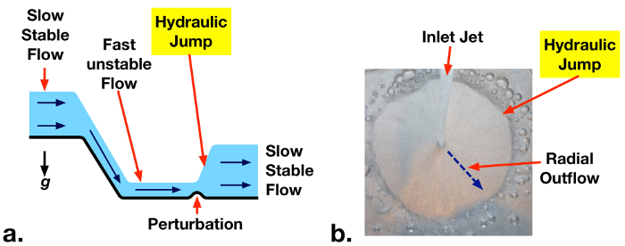
Figura 1: a. hidráulico salto que ocurre aguas abajo de un vertedero debido a una perturbación ligera para un flujo inestable de alta velocidad. b. ejemplo de salto hidráulico en la salida radial de agua de un grifo doméstico.

Principles

En flujos de canal ancho abierto, líquido se limita sólo por un límite sólido inferior y su superficie superior está expuesto a la atmósfera. Un análisis del volumen de control se puede realizar en una sección de un flujo de canal abierto para equilibrar la entrada y salida de transporte de masa y momentum (Fig. 2). Si las velocidades se supone uniforme en la entrada y salida del volumen de control (V1 y V2 respectivamente) con correspondientes profundidades líquido H1 y H2, entonces una masa constante flujo de equilibrio reduce a:

Equation 1(1)

El x-análisis del impulso de dirección de este control volumen equilibra las fuerzas de presión hidrostática (debido a la profundidad de líquido) con las entrada y salida impulso caudales (ecuación. 2). Las fuerzas de presión actúan hacia el interior de los dos lados del volumen de control y son iguales a la gravedad específica del líquido (densidad líquido veces la aceleración de la gravedad: ρg), multiplicado por la profundidad media del líquido a cada lado (H12, H 22), multiplica la altura sobre la cual la presión actúa sobre cada lado (H1, H2). Esto resulta en la expresión cuadrática en el lado izquierdo de la ecuación 2. Las tasas de flujo de momentum a través de cada lado (ecuación 2, derecha) son iguales a las tasas de flujo de masa de líquido a través del volumen de control (en: Equation 2 , hacia fuera: Equation 3 ) multiplicado por las velocidades del fluido (V1, V2).

Equation 4(2)

Ecuación. 1 puede ser sustituida en la ecuación. 2 para eliminar V2. El número de Froude (Equation 5) puede también sustituirse, que representa la fuerza relativa del ímpetu fluido de entrada a las fuerzas hidrostáticas. La expresión resultante puede ser indicada como:

Equation 6(3)

Esta ecuación cúbica tiene tres soluciones. Uno es H1 = H2, que da el comportamiento normal de canal abierto (profundidad de entrada = salida de profundidad). Una segunda solución da un nivel líquido negativo, que es incontrolado y puede ser eliminado. La solución restante permite un aumento en profundidad (Salto hidráulico) o una disminución de la profundidad (depresión hidráulica), dependiendo de la entrada del número de Froude. Si la entrada del número de Froude (Fr1) es mayor que uno, el flujo se denomina supercrítico (inestable) y tiene alta energía mecánica (cinética + gravitacional energía potencial). En este caso, un salto hidráulico puede formar espontáneamente o debido a alguna perturbación al flujo. El salto hidráulico disipa energía mecánica en calor, reduce la energía cinética y aumentando ligeramente la energía potencial del flujo. La altura resultante de salida es dada por la ecuación 4 (una solución a la ecuación 3). No puede ocurrir una depresión hidráulica si Fr1 > 1 porque aumentaría la energía mecánica del flujo, violando la segunda ley de la termodinámica.

Equation 7(4)

La fuerza de saltos hidráulicos aumenta con la entrada de números de Froude. Fr1 aumenta, aumenta la magnitud de H2/h1 y una mayor parte de la energía cinética de entrada se disipa como calor [1].

Figure 2
Figura 2: Control de volumen de una parte de un flujo de canal abierto que contiene un salto hidráulico. Entrada y masa y ímpetu se indican las tasas de flujo por ancho de la unidad. Fuerzas hidrostáticas por ancho de la unidad indican en el diagrama inferior.

Procedure

Nota: Este experimento utiliza una relativamente potente bomba sumergible. La bomba debe conectarse solamente a un tomacorriente GFCI para reducir al mínimo los riesgos eléctricos. Asegurarse de que no hay otros dispositivos de aire acondicionado accionado están operando cerca del experimento. 1. fabricación de instalaciones de flujo de canal abierto y el tanque (ver diagrama y fotografía, Fig. 3) Corte longitudes de ~6.0 mm espesor x 9,5 cm de ancho claro hoja de acrílico con las siguientes longitudes: 2 × 15 cm, 2 × 25 cm, 1 × 34 cm, 1 × 41 cm (Fig. 3a). Se recomienda utilizar una mesa de sierra o cortadora láser para asegurar que los bordes son relativamente planos y las hojas tienen igual espesor. Corte los orificios en las esquinas inferiores de la derecha de las hojas de acrílico de dos 60 × 45 cm para montar el medidor de flujo (Fig. 3a). Corte un agujero en la parte superior derecha de la hoja frontal para instalar la válvula de control de flujo. Use cemento acrílico (p. ej., SCIGRIP 16) para adherir los paneles de acrílico como se indica en la figura 3a. Asegurar una ventilación adecuada y use guantes al manipular el cemento acrílico. Es útil para aplicar el adhesivo con una jeringa de aguja y utilice cinta adhesiva para colocar los paneles durante el curado. Permita que el cemento curar durante 24-48 horas. Instale el medidor de flujo en el panel frontal y fije con los tornillos suministrados. Instalar 1 NPT racores reductores ½ de NPT en los puertos de entrada y salida del medidor de flujo. Instalar ½ NPT a 0,5 pulg. diámetro interno de púas de la guarnición adaptadores para los accesorios. Instale una en 0,5. Identificación y una en 0,75. ID. de púas en la válvula de compuerta (control de velocidad de flujo). Adaptador de conexión el púas para la bomba sumergible con una longitud de unos 20 cm del tubo de modo que la manija de la válvula se alinee con el orificio en la parte superior derecha de la caja de acrílico (Fig. 3b-c). Introducir la bomba en el depósito inferior e instale la válvula para que el vástago de la válvula pasa a través del orificio de montaje y el mango está fuera de la caja (Fig. 3 c). Inserte un panel acrílico vertical cerca de la entrada de la instalación de flujo de modo que hay aproximadamente un 5,0 mm abertura por debajo de ella (Fig. 3b-c). Este componente actúa como la compuertay se puede levantar y bajar para controlar el flujo desde el depósito superior al canal. Llene el depósito superior ligeramente con una lana de acero inoxidable restregar. Esto ayuda a distribuir uniformemente el flujo de agua de entrada a través del canal. Conecte la salida de la válvula a la entrada del medidor de flujo con una longitud de tubería de plástico blando. Conecte la salida del medidor de flujo para el depósito superior con tubería plástica. Asegúrese de que la entrada de la tubería en el depósito superior está bien anclada para que no se balancee hacia fuera cuando la bomba se enciende. Llene el depósito inferior con agua. 2. realizar el experimento Medir la altura de la brecha por debajo de la puerta utilizando una regla y denotan el valor como H1. Encienda la bomba y ajustar el flujo mediante la válvula para diferentes caudales (5-15 l min-1). Use una regla para medir la profundidad de líquido aguas abajo de la puerta (H2) para cada caso. Observar cualitativamente las formas de los saltos hidráulicos que se forman en las tasas de flujo diferentes. Reloj para el caudal de umbral mínimo para la formación de un salto hidráulico. Más agudo, una mayor amplitud (H2 -H1), saltos si ocurren a tasas de flujo más altas. 3. Análisis de los datos Para cada caso de la tasa de flujo, calcular la velocidad de entrada, V1, de la tasa de flujo volumétrico. donde es la tasa de flujo de volumen y W es el ancho de canal. Evaluar la entrada de número de Froude () y la profundidad de líquido aguas abajo teórica para cada caso (ecuación. 4). Comparar estos valores con profundidades de medida salto aguas abajo. Figura 3 : a. esquema y dimensiones de instalación estructura. b. diagrama de flujo de salto hidráulico instalación. c. etiquetadas fotografía experimental Centro.

Results

Upstream Froude numbers (Fr1) and measured and theoretical downstream depths are summarized in Table 1. The measured threshold inlet flow rate for formation of a hydraulic jump corresponds to Fr1 = 0.9 ± 0.3, which matches the theoretical value of 1. At supercritical flow rates (Fr1 > 1) predicted downstream depths match theoretical values (Eqn. 4) within experimental uncertainty.

Table 1 – Measured upstream Froude numbers (Fr1) and downstream liquid depths for H1 = 5 ± 1 mm

Liquid Flow Rate

(Equation 9, l min-1)

Upstream Froude Number (Fr1) Measured Downstream Depth (H2) Predicted Downstream Depth (H2) Notes
6.0   ± 0.5 0.9 ± 0.3 5 ± 1 5 ± 1 Threshold Froude number for hydraulic jump
11.0 ± 0.5 1.7 ± 0.5 11 ± 1 10 ± 2
12.0 ± 0.5 1.9 ± 0.6 12 ± 1 11 ± 2
13.5 ± 0.5 2.1 ± 0.6 14 ± 1 13 ± 2

Photographs of the hydraulic jumps from the above cases are presented in Fig. 4. No jump is observed for Equation 9 = 6.0 l min-1 (Fr1 = 0.9). Jumps are observed for the two other cases with Fr1 > 1. A stronger, higher amplitude, jump is observed at the higher flow rate supercritical case.

Figure 4
Figure 4: Photograph of hydraulic jumps, showing critical condition (no jump, Fr1 = 0.9) and jumps at Fr1 = 1.9, 2.1.

Applications and Summary

This experiment demonstrated the phenomena of hydraulic jumps that form at supercritical conditions (Fr > 1) in open channel flows. An experimental facility was constructed to observe hydraulic jump phenomena at varying flow rates. Downstream liquid depths were measured and matched with theoretical predictions.

In this experiment, the maximum reported inlet Froude number was 2.1. The pump was rated to deliver significantly higher flow rates, but resistance in the flow meter limited measurable flow rates to ~14 l min-1. In future experiments, a pump with a greater head rating or a lower pressure drop flow meter may enable a broader range of studied conditions.

Hydraulic jumps are often engineered into hydraulic systems to dissipate fluid mechanical energy into heat. This reduces the potential for damage by high velocity liquid jetting from spillways. At high channel flow velocities, sediment can be lifted up from streambeds and fluidized. By reducing flow velocities, hydraulic jumps also reduce the potential for erosion and scouring around pilings. In water treatment plants, hydraulic jumps are sometimes used to induce mixing and aerate flow. The mixing performance and gas entrainment from hydraulic jumps can be observed qualitatively in this experiment.

For all of these applications, momentum analyses across hydraulic jumps, as discussed here, are key tools for predicting hydraulic system behavior. Similarly, scale model experiments such as those demonstrated in this project, can guide the design of open-channel flow geometries and hydraulic equipment for large-scale engineering applications.

References

  1. Cimbala, Y.A. Cengel, Fluid Mechanics Fundamentals and Applications, 3rd edition, McGraw-Hill, New York, NY, 2014.

Transcript

A hydraulic jump is a phenomenon that occurs in fast-moving open flows when the flow becomes unstable. When a jump occurs, the height of the liquid surface increases abruptly resulting in an increased depth and decreased average flow velocity downstream. An important side effect of this phenomenon is that much of the kinetic energy in the upstream flow is dissipated as heat. Although hydraulic jumps often arise naturally, such as in rivers or the flow into a household sink, they are also purposely engineered into large waterworks to minimize erosion, or increase mixing. This video will illustrate the principles behind hydraulic jumps in a straight channel and then demonstrate the phenomenon experimentally using a small-scale open channel flow facility. After analyzing the results, some applications of hydraulic jumps will be discussed.

Consider the flow in a wide, straight section of an open channel where a hydraulic jump occurs and construct a control volume on a sluice around the jump. If the flow velocity is uniform at the inlet and outlet, conservation of mass yields a simple relation between upstream and downstream fluid depths. Depth multiplied by velocity is constant. A second relation can be found by considering conservation of momentum. Mass transported across the input and output carries momentum with it equal to the corresponding mass flux multiplied by the flow velocity. Hydrostatic forces on the surface of the control volume also contribute to the momentum balance and must be included. These forces are equal to the average pressure on the surface multiplied by the area. At this point, it is useful to introduce the Froude number, a dimensionless quantity named after the English engineer and hydrodynamicist, William Froude. The Froude number characterizes the relative strength of fluid momentum to hydrostatic forces. Now, if the momentum relation is rewritten in terms of the Froude number, with the output velocity eliminated by substitution using the mass relation, the result is a cubic equation in terms of the ratio of downstream and upstream depths. This equation can be simplified by factoring out the trivial solution where the upstream and downstream depths are equal. The two remaining solutions are easily found using the quadratic equation, but the negative solution can be eliminated since it is non-physical. The remaining solution corresponds to an increase in depth, a hydraulic jump, or a decrease in depth, a hydraulic depression, based on the value of the upstream Froude number. If the upstream Froude number is greater than one, the flow has a high mechanical energy and is supercritical or unstable. A hydraulic depression cannot form in this regime because it would increase mechanical energy and violate the second law of thermodynamics. On the other hand, a hydraulic jump can form, either spontaneously or due to some disturbance in the flow. An input Froude number of one represents the minimum threshold for the onset of a hydraulic jump. Hydraulic jumps dissipate mechanical energy into heat, and significantly reduce the kinetic energy, while slightly increasing the potential energy of the flow. As the Froude number increases, so does the ratio of downstream to upstream depths and the amount of kinetic energy dissipated as heat. Now that we understand the principles behind hydraulic jumps, let’s examine them experimentally.

First, fabricate the open channel flow facility as described in the text. The facility has an upper and lower reservoir connected by an open channel. Water pumped from the lower reservoir is deposited in the upper reservoir with the flow rate controlled and measured by a valve and flow meter in line with the pump. Steel wool in the upper reservoir helps to evenly distribute the water across the width of the section, and the adjustable sluice gate controls the fluid depth as it enters the channel. After flowing through the channel, the fluid is deposited back into the lower reservoir. When the flow facility is assembled, set it up on a bench and remove any nearby electronic devices. Plug the pump into a GFCI outlet to minimize the risk of electrical shock, and then fill the lower reservoir with water. You are now ready to perform the experiment.

Adjust the sluice gate to approximately five millimeters. Measure the final height of the gap underneath the sluice gate using a ruler, and record this distance as the upstream flow depth, H1. When you are finished, turn on the pump and use the valve to maximize the flow rate without exceeding the scale on the flow meter. Use the ruler again to measure the fluid depth after the hydraulic jump. Record the flow rate, along with this second distance which is the downstream flow depth, H2. Before continuing, observe the shape of the hydraulic jump. You should notice larger, more abrupt transitions for higher flow rates, and smaller, more gradual transitions for lower flow rates. Now, repeat your measurements and observations for successively lower flow rates. Try to determine the minimum threshold flow rate for the formation of a hydraulic jump. Once you have found the threshold flow rate, you are ready to analyze the results.

For each volumetric flow rate, you should have a measurement of the downstream fluid depth. The upstream depth is the same for all cases. Complete the following calculations for each measurement and propagate uncertainties along the way. First, determine the inlet flow velocity. Divide the volumetric flow rate by the channel width and upstream depth. Next, evaluate the upstream Froude number using the definition given before, and substituting in the acceleration due to gravity, as well as the upstream height and velocity. Now, use the Froude number and the non-trivial solution for the jump height to calculate the theoretical downstream depth. Compare the theoretical prediction with the measured downstream depth. At supercritical flow rates, the predictions match the measured depths within experimental uncertainty. Look at your results for the threshold flow rate. Within experimental uncertainty, the Froude number is one, as we anticipated from the theoretical analysis. The rate of mechanical energy loss through the hydraulic jump can also be calculated from these data. First, calculate the mechanical energy of the fluid flowing into the jump, which is the sum of kinetic and potential energy flow rates at the inlet. Now, determine the output energy rate in the same way, but with values at the outlet. The rate of mechanical energy dissipation to heat is the difference between the input and output rates. In this experiment, the energy loss rate can reach about 40% of the inlet energy, or higher. These results highlight the effectiveness of momentum analyses and scale model experiments for understanding and predicting the behavior of hydraulic systems. Now let’s look at some other ways hydraulic jumps are utilized.

Hydraulic jumps are an important natural phenomenon with many engineering applications. Hydraulic jumps are often engineered into hydraulic systems to dissipate fluid mechanical energy into heat. This reduces the potential for damage by high velocity liquid jetting from spillways. At high channel flow velocities, sediment can be lifted up from streambeds and fluidized. By reducing flow velocities, hydraulic jumps also reduce the potential for erosion and scouring around pilings. In water treatment plants, hydraulic jumps are sometimes used to induce mixing and aerate flow. The mixing performance and gas entrainment from hydraulic jumps can be observed qualitatively in this experiment.

You’ve just watched JoVE’s introduction to hydraulic jumps. You should now understand how to use a control volume approach to predict the flow behavior, and how to measure this behavior using an open channel flow facility. You’ve also seen some practical uses for engineering hydraulic jumps in real applications. Thanks for watching.

Tags

Cite This
JoVE Science Education Database. JoVE Science Education. Hydraulic Jumps. JoVE, Cambridge, MA, (2023).