JoVE Science Education
Chemical Engineering
This content is Free Access.
JoVE Science Education Chemical Engineering
Vapor-liquid Equilibrium
  • 00:07Overview
  • 01:36Principles of Vapor-liquid Equilibrium
  • 05:15Priming the VLE System
  • 06:00Running VLE Experiments
  • 07:52Results
  • 09:33Applications
  • 11:09Summary

Dampf-Flüssigkeits-Gleichgewicht

English

Share

Overview

Quelle: Michael G. Benton und Kerry M. Dooley, Department of Chemical Engineering, Louisiana Landesuniversität, Baton Rouge, LA

Dampfflüssigkeit Gleichgewicht ist in technischen Anwendungen wie Destillation, Umgebungsmodellierung und allgemeine Prozessgestaltung von größter Bedeutung. Verständnis der Interaktionen der Komponenten in einer Mischung ist sehr wichtig in der Entwicklung, Betrieb und analysieren diese Separatoren. Der Aktivität-Koeffizient ist ein ausgezeichnetes Werkzeug für im Zusammenhang mit molekularen Wechselwirkungen zu Mischungszusammensetzung. Finden die molekulare Interaktion Parameter ermöglicht zukünftige Vorhersage der Tätigkeit Koeffizienten für eine Mischung mit Hilfe eines Modells.

Dampfflüssigkeit Gleichgewicht ist ein kritischer Faktor für gemeinsame Prozesse in der chemischen Industrie, wie die Destillation. Destillation ist der Prozess der Trennung von Flüssigkeiten durch ihren Siedepunkt. Eine flüssige Mischung in einer Destillationseinheit oder Spalte gefüttert, dann gekocht. Dampfflüssigkeit Gleichgewichtsdaten eignet sich zum bestimmende wie Flüssigkeitsgemischen trennen werden. Da die Flüssigkeiten unterschiedliche Siedepunkte haben, wird eine Flüssigkeit in Dampf kochen und steigen in der Spalte, während die andere als Flüssigkeit bleiben und durch das Gerät entleeren. Der Prozess ist sehr wichtig in den unterschiedlichsten Branchen.

In diesem Experiment die Tätigkeit Koeffizienten der Mischungen unterschiedlicher Zusammensetzung von Methanol, Isopropanol und deionisiertes Wasser erhält man mit einem Dampfflüssigkeit Gleichgewicht Gerät und Gaschromatographen. Zusätzlich werden die binäre Interaktion Parameter des Systems mit Wilsons Gleichung und die Tätigkeit Koeffizienten bestimmt werden.

Principles

Dampfflüssigkeit Gleichgewicht ist ein Zustand, in dem eine reine Komponente oder Mischung in Flüssigkeit und Dampf Phasen mit mechanischen und thermischen Gleichgewicht und kein net Stoffaustausch zwischen den beiden Phasen vorhanden ist. Dampf und Flüssigkeit werden durch Schwerkraft und Hitze (Abbildung 1) getrennt. Die flüssige Mischung wird in das System eingefügt, die in einem Vakuum Zustand mit einer Vakuumpumpe genommen wird. Der Dampf wird kondensiert und zum Mischen mit der Flüssigkeit, die dann zurück in die kochende Kammer übergeben wird zurückgegeben. Unterschiede in der Siedepunkt resultiert eine Trennung des Gemisches. Der Siedepunkt des Wassers ist höher als die der zusätzlichen Komponenten, so dass die flüchtigen Bestandteile beginnen zu verdampfen.

Figure 1
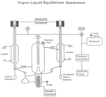
Abbildung 1: Darstellung des Apparates

Eine Tätigkeit Koeffizient ist definiert als das Verhältnis der Vergänglichkeit einer Komponente in einer tatsächlichen Mischung, die Vergänglichkeit eine ideale Lösung für die gleiche Zusammensetzung. Vergänglichkeit ist eine Eigenschaft verwendet, um Unterschiede zwischen chemischen Potentialen bei standard Staaten zeigen. Vapor Phase Fugacities in Bezug auf die Vergänglichkeit Koeffizienten ausgedrückt werden können [φ: fichV = φich yich fich0V ], mit yich = ich Mol Bruchteil in der Dampfphase und fich0V = Dampf-Standard Vergänglichkeit der Staat (die Vergänglichkeit der reinen Komponente Dampf bei T und P). Für niedrige Drücke, wie dieses Experiment, φich = 1 und fich0V = P. Liquid Phase Fugacities eine Tätigkeit Koeffizient γichausgedrückt werden können: fichL = γi xich fich 0 L , mit xich = Mol Teil i in der flüssigen Phase, und fich0 L = standard flüssig Vergänglichkeit.

Bei der Sättigungsdruck (Pichs) von diesem T wäre der reinen Komponente flüssig Vergänglichkeit Pis, da die reine Dampf und Flüssigkeit im Gleichgewicht sind. Da flüssige Fugacities nur schwache Funktionen des Drucks sind, können wir die reinen Komponente flüssig Vergänglichkeit T und P (fich0 L) als Pichs, annähern, solange der Unterschied zwischen Pichs und P nicht groß ist. Diese Annäherung ist in der Regel “vernachlässigen die Poynting-Korrektur” genannt. Wenn Experimentatoren ein VLE-Gerät verwenden, um die Kompositionen von Dampf und Flüssigkeit zu messen, die im Gleichgewicht sind, Experimentatoren können direkt berechnen die Tätigkeit Koeffizienten zur Maßnahme auch P und T. T muss gemessen werden, um festzustellen, PichS für alle ich.

Das Herz des Geräts VLE, in dieses Experiment verwendet, um Kompositionen von Mischungen, zu bestimmen ist eine Cottrell-Pumpe, die “kochende Flüssigkeit in eine gut isolierte Gleichgewicht Kammer spuckt”. Zwei magnetisch betätigten Probenahme-Ventile ermöglichen nach Abzug der flüssigen und kondensierten Dampf Proben. Ein großes Reservoir hilft, um Druckstöße im System als die on / off Ventil Steuerschalter und von Schwankungen durch die Cottrell-Pumpe zu dämpfen. Ein langsames Leck kann verwendet werden, um ein Gleichgewicht zwischen dem Kurs des Entzugs der Luft und die Rate für die Eingabe der Luft, um einen konstanten Druck, erhalten nach Bedarf erstellen.

Eine vergleichbare Möglichkeit für Dampfflüssigkeit Gleichgewicht zu lösen ist, eine Vielzahl von Modellen verwenden. Raoult Gesetz, Dalton Gesetz und das Gesetz von Henry sind alle theoretischen Modellen, die die Dampfflüssigkeit Gleichgewicht Konzentrationsdaten finden können. Alle drei Modelle beziehen sich auf die Verhältnismäßigkeit der Partialdrücke, Gesamtdruck und Maulwurf Brüche von Stoffen. Wilsons Gleichung ist nachgewiesen worden, genaue mischbaren Flüssigkeiten, werden zwar nicht übermäßig komplex. Darüber hinaus enthält Wilsons Modell Tätigkeit Koeffizienten um Abweichung vom idealen Werte zu berücksichtigen.

Procedure

1. Grundieren das system Entlüften mit dem Vent/3-Wege Regelventil montiert auf dem Rahmen des Apparates, VLE und (falls erforderlich) durch Ablassen von Flüssigkeit aus dem System heraus in einem Abfall Kolben. Entfernen Sie die Probenröhrchen und ersetzen durch saubere Rohre (bei Bedarf). Die Flüssigkeit wird nicht vollständig aus dem System ablassen. Für den ersten Lauf der Experimente, etwa durch das Eingangsventil mit einer Mischung aus nachfüllen (Vol-%) 50 % Methanol, Isopropanol 30 % und 20 % Wasser. Für die zweite Woche mit etwa 25 % Methanol, Isopropanol 45 % und 30 % Wasser nachfüllen. Für die dritte Woche füllen Sie mit welcher Flüssigkeit müssen Sie wiederholen. Die flüssigen Gesamtkapazität beträgt ca. 130 cm3. Füllen Sie mit Flüssigkeit bis knapp unter die Stelle wo die Cottrell-Pumpe mit Vakuum Jacke schneidet. Zu wenig Flüssigkeit bewirkt, dass das System erfordern sehr hohe kochende Raten zu bekommen genug Flüssigkeit zu “spucken” (wenn Flüssigkeit erscheint während des Kochens intensiv). Verwenden Sie einen Becher und gießen Sie die Flüssigkeit in den Zusatz-Anschluss an der Spitze der Kammer Gleichgewicht. In der Nähe des Hafens. Überprüfen Sie den Luftdruck mit Quecksilber Manometer an der Wand. Passen Sie die “Null” auf dem digitalen Manometer entsprechen (falls erforderlich). Wechseln Sie das Dreiwege Entlüftungsventil zur “Kontrolle” und starten Sie die Vakuumpumpe und Druckregler. Öffnen Sie Drosselklappe auf dem Druck-Controller mehrere Umdrehungen und beobachten Sie den Druck schnell fallen. Beobachten Sie den Druck auf das digitale Manometer. Setzen den Druck Satz-Kontrollpunkt auf der Druckregler erhalten ~ 700 mm Hg. hören für das Anklicken des Steuerventils. Wenn der Kontrollpunkt erreicht ist, wird der Lärm von der Vakuumpumpe hörbar anders sein. Zu diesem Zeitpunkt eröffnete mit der Drosselklappe mehrere Umdrehungen, jedes Mal, wenn das Regelventil öffnet, zuviel Luft wird weggeworfen, die Vakuumpumpe und der Druck taucht unter 700 mm vor langsam erholt. Schließen Sie die Drosselklappe vollständig, dann öffnen Sie ihn über ½ Umdrehung. Warten auf das Steuerventil zu beginnen, wenn Sie erneut klicken, dann schließen Sie die Drosselklappe in kleinen Schritten, bis der Druck nur ~0.5 MmHg schwankt oder weniger, wenn das Ventil geöffnet ist. Anpassungen Sie geringfügige an den Kontrollpunkt oder das Leck-Ventil um zu sehr in der Nähe von 700 MmHg halten. Sobald die Mischung innerhalb von ± 10 MmHg von 700 MmHg ist, schalten Sie die Heizung, Heizwasser Mantel macht, Kondensator und Magnetrührer. Versuchen Sie 25-30 % Heizleistung und 1,5 bis 2 Umdrehungen Mantel macht zu starten. Das Gerät erfordert 20 min oder weniger zum Ansatz Gleichgewicht. Passen Sie halten Sie den Druck während dieser Zeit an. 2. Durchführung des Experiments Beim Kochen, die Cottrell-Pumpe startet Flüssigkeit zu spucken und Flüssigkeit tropft zurück in die kochende Kammer gesehen werden kann. Kondensierten Dampf erfordert mehr angezeigt werden. Wenn Gleichgewicht erreicht wird, sollten Experimentatoren stetig tropft der kondensierte Dampf sehen (2 – 3 Tropfen/s) und kehrte Flüssigkeit (2 – 3 Tropfen/s). Die Temperatur sollte stabil ± 0,03 º c und der Druck sollte bei 700,0 ± 0,5 MmHg stabil sein. Wenn diese Bedingungen für mindestens 2 Minuten (oder so) aufgestellt wurden, wird Gleichgewicht erreicht. Öffnen Sie die Magnetventile (markiert “1” und “2” auf dem Controller) 4 oder 5 Mal jede lange genug, um über 0,5 cm3 Flüssigkeit in jedem Beispiel Röhrchen sammeln, und schließen Sie die Rohre. Wenn ein Ventil nicht auf die Schaltfläche “reagiert, versuchen Sie, spiegeln den ein-/Ausschalter für den Controller ausschalten dann auf. In diesem ersten Beispiel wird verwendet, um die Rohre und Liefersystem waschen und werden verworfen. Waschen ersetzt keine verbleibenden chemischen auf den Seiten der Rohre mit der gleichen Chemikalie, die gemessen wird, ist, so daß es wird keinen Einfluss auf die Zusammensetzung des Tests. Schalten Sie einen Moment das Gerät an den Heizkörper, warten 30 s für das Kochen zum Abklingen, dann entlüften Sie das System mit 3-Wege Ventil/Regelventil. Entfernen Sie die Probenröhrchen, schwenken ein paar Mal, dann steckt sie in den Abfall Pot. Einbauen Sie die Probenröhrchen auf dem System wieder, drehen Sie das Entlüftungsventil zurück zu “kontrollieren”, schalten das Gerät wieder auf die Heizung und warten auf Gleichgewicht wiederhergestellt werden. Dies dauert nur ein paar Minuten, wenn der Apparat nicht kühlt. Ein leichter Unterschied in der Temperatur kann beobachtet werden, wenn das Gleichgewicht wieder hergestellt ist. Dies kann aufgrund einer leichten Störung der Gesamtkomposition durch Abtastung sein. Sobald das Gleichgewicht wieder hergestellt ist, nehmen Sie zwei neue Proben. Haben Sie zwei beschriftete Fläschchen mit neuen Septen bereit. Schalten Sie nach der Einnahme von ~0.5 cm3 Proben in jedem Röhrchen wieder die Heizung entlüften Sie, entfernen Sie die Probenröhrchen und gießen Sie sie in das Fläschchen. Die Küvetten mit dem Deckel und ggf. die Probenröhrchen durch saubere Rohre ersetzen. Bereiten Sie bei der Analyse der Proben eine neue Probe vor. Entleeren Sie ~ 15 cm3 Flüssigkeit in ein Becherglas oder Fläschchen. ~ 20 cm3 reines Methanol oder 50/50 Methanol/Isopropanol durch den Probenport hinzufügen. Dies wird eine neue Gesamtkomposition geben. Achten Sie darauf die Probenröhrchen sind völlig leer, dann schließen Sie das System aus, wechseln Sie das Entlüftungsventil zur “Kontrolle” und die Heizung wieder einzuschalten. Wenn Sie schnell arbeiten, wird Gleichgewicht schnell wiederhergestellt werden. Beachten Sie, daß es eine Temperaturdifferenz aus dem vorherigen Beispiel. Wiederholen Sie die Gleichgewichtherstellung und Stichprobenverfahren als vor, daran zu denken, nehmen eine Probe zu waschen, und dann die endgültige Stichprobe. Die Experimente durch das Hinzufügen von Komponenten weiter. Zwölf Datenpunkte sind ausreichend, um die Tätigkeit Koeffizienten und (ungefähr) die binäre Interaktion Koeffizienten zu bestimmen. 3. Herunterfahren das system Schalten Sie die Heizung aus. Wenn das Gerät beginnt zu kühlen, schalten Sie das Rührwerk und Kondensator Wasser. Das System auf den atmosphärischen Druck zurückzusenden; Stellen Sie den Regler > 1020 Mbar, schließen Sie die Drosselklappe, legen Sie das Dreiwege Ventil entlüften und öffnen Sie das Ventil am Tank. Atmosphärischer Druck erreicht hat, schalten Sie die Pumpe. Lassen Sie die Flüssigkeit aus dem Behälter ab, bis es das Niveau des Ventils erreicht, aber überlassen Sie den Rest der Flüssigkeit im Behälter. Schließen Sie das 3-Wege-Ventil. 4. Analyse Nicht-lineare Regression und ein standard Summe der quadrierten Residuen Zielfunktion, Verwendung der Tätigkeit Koeffizienten berechnet aus den Rohdaten bilden die 6 Konstanten für die ternären Wilson-Gleichung (siehe unten), für dieses System. Beurteilung der Qualität der Passung durch grafische Methoden und Informatik die durchschnittliche prozentuale relative Abweichungen (APRD), die durchschnittliche eignen Fehler X 100. Konvergieren Sie auf die wahren optimale Werte aus mehreren unterschiedlichen Richtungen im Parameterraum Antwort mithilfe einer faktoriellen Methode für die anfänglichen Vermutungen. Berechnen Sie die Genauigkeit der Messungen GC, indem ausreichend repliziert eine GC-Probe um relative Genauigkeiten nach t-Kenngröße zu bestimmen, und verwenden Sie die Genauigkeiten um zu bestimmen, ob Sie akzeptieren / ablehnen einer bestimmten GC-Messung durch geeignete Hypothesentest. Die relative Genauigkeiten der GC-Messung an der APRDs zu vergleichen und diskutieren. Auch berichten die absolute Genauigkeiten von Druck und Temperatur Manometer – diese einmal pro Tag zu bestimmen.

Results

The activity coefficients of the data do not show significant deviations from a mean value for each component (Table 1). This is as expected because for intermediate component compositions there are not large variations. However, components near 1 have γ's near 1. Low composition components have high γ's. Components highest in concentration in a mixture which will have a reduced deviation, therefore it will be closer to ideal (γ = 1). Components with lower concentrations in a mixture will have higher deviations, so their γ's will be greater than 1.

Table 1

Table 1: Results of each sampling of the experimental data.

The data were fit to Wilson model parameters and the coefficients were calculated (Table 2). A simple reduction in the sum of squared residuals between experimental and Wilson equation (1) activity coefficients was used. This was achieved using Excel's solver function. The parity plot shown relates the Wilson's Equation model activity coefficients to the experimentally found activity coefficients. The experimental activity coefficients were calculated and graphically compared to the calculated model coefficients.

Table 2

Table 2: Results of fitting the data to the Wilson model parameters.
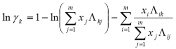
Equation 1 (1)

The parameter values found were the best fit (Table 3). Ideally the correlation is along the y=x line; however, a significant correlation resembling the ideal scenario was found (Figure 2). The activity coefficients of the data did not show significant deviations from a mean value for each component, as expected. A reduction in the sum of squared residuals between experimental and Wilson equation activity coefficients was used with Excel's solver function. The parity plot relates the Wilson's Equation model activity coefficients to the experimentally found activity coefficients.

Table 3

Table 3: Model parameters with water (a), MeOH (b), and IPA (c). The experimental values are compared to expected values.

Figure 2
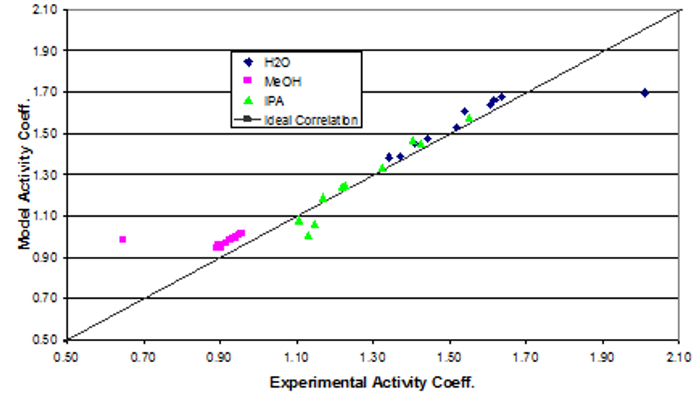
Figure 2: Depiction of the correlation between the experimental activity coefficients and the model activity coefficients.

Applications and Summary

This experiment demonstrated the equilibration of methanol – isopropanol – water vapor-liquid mixtures at a constant P = 700 mm Hg and how to measure temperature and composition and calculate activity coefficients. The activity coefficients of the data did not significantly deviate from a mean value for each component, as expected. A reduction in the sum of squared residuals between experimental and Wilson equation activity coefficients was used with Excel's solver function. The parity plot relates the Wilson's Equation model activity coefficients to the experimentally found activity coefficients.

In the petroleum industry, distillation is the primary process for separation of petroleum products. Many oil refineries use distillation for crude oil1. Light hydrocarbons are separated from heavier particles, separating based on boiling points1. Heavy materials like gas oils collect in the lower plates, while light materials like propane and butane rise up1. Hydrocarbons, such as gasoline, jet, and diesel fuels, are separated1. This process is often repeated many times to fully separate and refine the products1. Refineries run these processes at steady state, constantly creating new products at maximum capacity, so efficiency is key1. Chemical engineers working on these processes focus on optimizing the efficiency of the production1.

Tray distillation columns are also used to separate a variety of chemical products. Ethanol is one such product. Through closely related processes, a variety of products such as fuel-grade ethanol, beer, and liquor can all be distilled2. Specific amounts of alcohol can be separated from water in order to create a specific proof2. This process is limited to reducing the percentage of water in the product, but cannot completely eliminate it2. In order to remove water completely, azeotropic distillation is required, which uses extractor chemicals to separate water from ethanol2.

References

  1. About the Refinery." Processing & Refining Crude Oil. Chevron.com, n.d. Web. 17 Nov. 2016.
  2. Madson, PW. Ethanol Distillation: The Fundamentals. Cincinnati: Katzen International, n.d. Print. Accessed from Web. 01 Oct. 2016.

Transcript

Understanding the distribution of chemical components in both the vapor and liquid phase, called vapor-liquid equilibrium is essential to the design, operation, and analysis of many engineering processes. Vapor-liquid equilibrium or VLE is a state at which a pure component or mixture exists in both the liquid and vapor phases. The phases are at equilibrium meaning that there were no changes in the macroscopic properties of the system over time. Single component VLE is simple to visualize. Take for example water which is at equilibrium in the vapor and liquid phase at 100 degrees Celsius and one atm. Above this temperature water is a vapor. Below it, water is a liquid. However, engineers generally encounter processes with mixtures in equilibrium making the analysis of VLE more complex and therefore essential to process design. This video will illustrate the principles behind vapor-liquid equilibrium of mixtures and demonstrate how to analyze the VLE of a mixture in the laboratory. Finally, some applications of VLE in the chemical engineering field will be introduced.

When a heated mixture is in a vapor-liquid equilibrium, the vapor and liquid phases generally do not have the same composition. The substance with the lower boiling point will have a higher concentration in the vapor than the substance with the higher boiling point. Thus, engineers refer to components in each phase by their mole fraction where xi is the mole fraction of species i in the liquid and yi is the mole fraction of species i in the vapor phase. This relationship is often depicted using an xy curve like the one shown here for a mixture of two components which illustrates the relationship between each component in each phase. A starting point for all VLE calculations is the simple equilibrium criterion where the fugacity of the species in the vapor equals the fugacity of the species in the liquid. Fugacity is a property related to the exponential difference between the real and ideal gas Gibbs energies. The vapor phase fugacity is equal to the mole fraction of species i in the vapor phase times the pure component vapor fugacity. The expression can be simplified as the pure component vapor fugacity is approximately equal to pressure at low pressure. Liquid phase fugacities are expressed in terms of an activity coefficient, gamma. The activity coefficient is defined as the ratio of a component’s fugacity in an actual mixture to the fugacity of an ideal solution of the same composition. At the saturation vapor pressure the pure component liquid fugacity would equal the saturation vapor pressure because the pure vapor and liquid are in equilibrium there. Finally, since the liquid and vapor fugacities are equal, we can further simplify the relationship as shown which is also known as Raoult’s law. The saturation vapor pressure is often calculated using the Antoine equation where the constants A, B, and C are species-specific and can be found in the literature. Thus, if we measure the compositions of the vapor and liquid which are in equilibrium, we can directly calculate the activity coefficients by measuring temperature and pressure and therefore the saturation vapor pressure. In this experiment a ternary mixture of methanol, isopropyl alcohol and water will be investigated. Various compositions of the mixture are boiled in a VLE apparatus and the lower boiling point components vaporize and are collected in a separate container while the liquid gathers back into the initial sample vessel. Once equilibrium is reached, the liquid and condensed vapor fractions are collected and analyzed with gas chromatography. Using temperature and the liquid and vapor mole fractions the activity coefficients can be calculated. Now that you’ve been introduced to the concepts of VLE and the testing apparatus, let’s see how to carry out the experiment in the laboratory.

To start, drain any liquid out of the system into a waste flask. Keep in mind that the liquid may not completely drain. For the first run add a mixture of 50% methanol, 30% IPA and 20% water through the opening at the top. After filling the mixture, turn on the heater power and condenser water. The apparatus will require roughly 20 minutes to approach equilibrium. The system is now ready to begin the experiment.

When the sample begins boiling, release the stopper to vent the inert outlet of the system. Condensed vapor will start collecting. When equilibrium is reached, steady drips of condensed vapor and returns liquid should be observed. With the temperature stable to within 0.3 degrees for 10 minutes, collect about 1/2 milliliter of liquid in sample vials from both the condensed vapor and the boiling liquid. Drain the condensed vapor from the last sample. Then add a new sample consisting of either 20 milliliters of pure methanol or 50-50 methanol-isopropanol through the sample port. This will give a new overall composition. Reestablish the equilibrium as performed before, however expect a temperature difference from the previous sample. Repeat the equilibration and sampling procedure as before, and then collect the sample to be analyzed. Continue the experiment using different mixtures of the three components. 12 points are sufficient to determine the activity coefficients and the binary interaction coefficients. When all the mixtures have been run, shut down the system by turning off the heaters. When the apparatus begins to cool, shut off the condenser water. Finally measure the composition of each liquid and vapor sample with the gas chromatograph or GC.

Using the system temperature and the liquid and vapor mole fractions acquired from GC, calculate the activity coefficients. This first requires that the saturation pressure is calculated using the Antoine equation where the constants A, B and C for each component can be found in the literature. Now we can use the calculated activity coefficients to correlate the data to a model. We will use the Wilson equation for a ternary mixture which accounts for deviations from ideality in a mixture. The nine lambda constants are the Wilson constants which equal one when i equals j. For each ij pair, there are two different constants. Use a nonlinear regression and a standard sum of squares residual function to determine the six remaining Wilson constants using the mole fraction data from the experiment. The Wilson constants are then used to determine the expected activity coefficients for each component of each sample. Here we show the modeled activity coefficient plotted against the experimental activity coefficients. Ideally, the modeled and experimental activity coefficients would fall along the y equals x line. As you can see in general, the modeled and experimental values fit along this line showing that the model is a good fit to the real system.

Understanding and manipulating the vapor-liquid equilibrium of mixtures is a vital component to a range of processes especially separations. Distillation columns separate mixtures based on their volatility with different compositions of each component in the liquid and vapor phrases on each tray. The more volatile component is vaporized and collected at the top of the column, while the less volatile component remains liquid and is collected at the bottom. VLE data of the components of the mixture is used to determine the number of trays needed to achieve separation in a distillation column. This helps engineers optimize the separation process while keeping operating costs low. Another valuable separation technique using VLE is flash separation. Flash separation is based on the fact that a liquid at a pressure equal to or greater than its bubble point pressure flashes meaning that it partially evaporates when the pressure is reduced. The feed is preheated thus consisting of some liquid and some vapor in equilibrium. It then flows through a pressure reducing valve into the separator. The degree of vaporization and therefore the amount of the solute in the vapor or liquid phases depends on the initial state of the feed stream.

You’ve just watched Jove’s introduction to vapor-liquid equilibrium. You should now understand the concepts behind VLE, how it’s measured in the laboratory, and some of its uses in engineering processes. Thanks for watching.

Tags

Cite This
JoVE Science Education Database. JoVE Science Education. Vapor-liquid Equilibrium. JoVE, Cambridge, MA, (2023).