Vapor-liquid equilibrium is a state in which a pure component or mixture exists in liquid and vapor phases, with mechanical and thermal equilibrium and no net mass transfer between the two phases. Vapor and liquid are separated by gravity and heat (Figure 1). The liquid mixture is inserted into the system, which is put into a vacuum state with a vacuum pump. The vapor is condensed and returned to mix with the liquid, which is then passed back to the boiling chamber. Differences in the boiling point results in some separation of the mixture. The boiling point of water is higher than that of the added components, so the volatile components begin to evaporate.
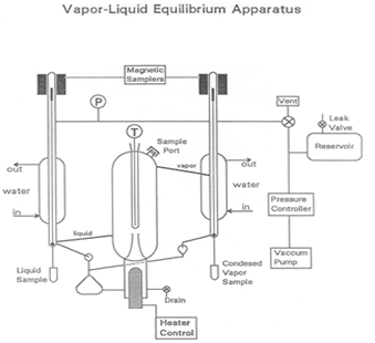
Figure 1: A depiction of the apparatus
An activity coefficient is defined as the ratio of a component's fugacity in an actual mixture to the fugacity of an ideal solution of the same composition. Fugacity is a property used to show differences between chemical potentials at standard states. Vapor phase fugacities can be expressed in terms of a fugacity coefficient [φ: fiV = φi yi fi0V ], with yi = mol fraction of i in the vapor phase, and fi0V = the vapor standard state fugacity (the fugacity of pure component vapor at T and P). For low pressures, as in this experiment, φi = 1 and fi0V = P. Liquid phase fugacities can be expressed in terms of an activity coefficient γi: fiL = γi xi fi0L , with xi = mol fraction of i in the liquid phase, and fi0L = the liquid standard state fugacity.
At the saturation pressure (Pis) of this T, the pure component liquid fugacity would be Pis, because the pure vapor and liquid are in equilibrium. Since liquid fugacities are only weak functions of pressure, we can approximate the pure component liquid fugacity at T and P (fi0L) as Pis, as long as the difference between Pis and P is not large. This approximation is usually called "neglecting the Poynting correction". If experimenters use a VLE apparatus to measure the compositions of the vapor and liquid which are in equilibrium, experimenters can directly calculate the activity coefficients provided to also measure P and T. T must be measured to determine PiS for all i.
The heart of the VLE device, used in this experiment to determine compositions of mixtures, is a Cottrell pump which "spits" boiling liquid into a well-insulated, equilibrium chamber. Two magnetically operated sampling valves allow for withdrawal of liquid and condensed vapor samples. A large reservoir helps to dampen pressure pulses in the system as the on-off control valve switches, and from fluctuations caused by the Cottrell pump. A slow leak can be used to create a balance between the rate of withdrawal of air and the rate of input of air to maintain a constant pressure, if necessary.
A comparable way to solve for vapor-liquid equilibrium is to use a variety of models. Raoult's law, Dalton's law, and Henry's law are all theoretical models that can find the vapor-liquid equilibrium concentration data. All three models are related to the proportionality of partial pressures, total pressure, and mole fractions of substances. Wilson's equation has been proven to be accurate for miscible liquids, while not being overly complex. Additionally, Wilson's model incorporates activity coefficients to account for deviation from ideal values.
1. Priming the system
- Vent the VLE system using the vent/control 3-way valve mounted on the frame of the apparatus, and (if necessary) by draining liquid out of the system into a waste flask.
- Remove the sample tubes and replace with clean tubes (if necessary). The liquid will not completely drain out of the system.
- For the first run of experiments, refill through the input valve with a mixture of roughly (vol %) 50% methanol, 30% isopropanol and 20% water. For the second week, refill with roughly 25% methanol, 45% isopropanol and 30% water. For the third week, refill with whatever liquid you need to repeat. The total liquid capacity is approximately 130 cm3.
- Fill with liquid to just below the spot where the Cottrell pump intersects with the vacuum jacket. Too little liquid will cause the system to require very high boiling rates to get enough liquid to "spit" (when liquid pops while boiling intensely).
- Use a beaker and pour the liquid into the addition port at the top of the equilibrium chamber. Close the port.
- Check the barometric pressure with the mercury manometer on the wall. Adjust the "zero" on the digital pressure gauge to match (if necessary).
- Switch the three-way vent valve to "control" and start up the vacuum pump and pressure controller.
- Open the throttle valve on the pressure controller several turns and observe the pressure rapidly drop. Watch the pressure on the digital pressure gauge.
- Set the control pressure set-point on the pressure controller to obtain ~ 700 mm Hg. Listen for clicking of the control valve. Once the control point is reached, the noise from the vacuum pump will be audibly different.
- At this point, with the throttle valve opened several turns, every time the control valve opens, too much air is dumped to the vacuum pump and the pressure dips below 700 mm before slowly recovering. Close the throttle valve completely, then open it about ½ turn.
- Wait for the control valve to begin clicking again, then close the throttle valve in small increments until the pressure fluctuates only ~0.5 mmHg or less when the valve is open. Make minor adjustments to the control point or the leak valve as necessary to maintain very near 700 mmHg.
- Once the mixture is within ±10 mmHg of 700 mmHg, turn on the heater power, heating mantle power, condenser water and magnetic stirrer. Try 25-30 % heater power and 1.5-2 turns mantle power to start. The apparatus will require 20 min or less to approach equilibrium. Keep adjusting the pressure during this time.
2. Running the experiment
- Upon boiling, the Cottrell pump will begin to spit liquid and liquid can be seen dripping back into the boiling chamber. Condensed vapor will require longer to appear. When equilibrium is reached, experimenters should see steady drips of condensed vapor (2 – 3 drops/s) and returned liquid (2 – 3 drops/s). The temperature should be stable to ± 0.03 ºC and the pressure should be stable at 700.0 ± 0.5 mmHg. When these conditions have been established for at least 2 min (or so), equilibrium is attained.
- Open the magnetic valves (marked "1" and "2" on the controller) 4 or 5 times each for long enough to collect about 0.5 cm3 of liquid in each sample tube, and close the tubes. If a valve does not respond to its button, try flipping the power switch for the controller off then on. This first sample will be used to wash the tubes and delivery system and will be discarded. Washing replaces any remaining chemical on the sides of the tubes with the same chemical that is being sampled, so it will not affect the composition of the test.
- Momentarily turn off the power to the heater, wait 30 s for the boiling to subside, then vent the system with the vent/control 3-way valve. Remove the sample tubes, swirl a few times, then dump them into the waste pot.
- Refit the sample tubes on the system, turn the vent valve back to "control", turn the power back on to the heater, and wait for equilibrium to be reestablished. This will only take a few min if the apparatus does not cool. A slight difference in temperature may be observed when equilibrium is re-established. This can be due to a slight disturbance of the overall composition due to sampling.
- Once equilibrium is re-established, take two new samples. Have two labeled vials with new septa ready.
- After taking ~0.5 cm3 samples in each tube again, turn off the heater, vent the system, remove the sample tubes and pour them into the vials. Cap the vials and replace the sample tubes with clean tubes if necessary.
- While analyzing the samples, prepare a new sample. Drain ~15 cm3 of liquid into a beaker or flask. Add ~20 cm3 of pure methanol or 50/50 methanol/isopropanol through the sample port. This will give a new overall composition.
- Be sure the sample tubes are completely empty, then close the system off, switch the vent valve to "control", and turn the heater back on. If working quickly, equilibrium will be re-established rapidly. Note that there should be a temperature difference from the previous sample.
- Repeat the equilibration and sampling procedure as before, remembering to take one sample to wash, and then take the final sample. Continue the experiments by adding component(s). Twelve data points are sufficient to determine the activity coefficients and (roughly) the binary interaction coefficients.
3. Shutting down the system
- Turn the heaters off. When the apparatus begins to cool, shut off the stirrer and condenser water.
- Return the system to atmospheric pressure; set the controller >1020 mbar, close the throttle valve, set the three-way valve to vent and open the valve on the tank.
- Once atmospheric pressure has been reached, shut off the pump. Drain the liquid from the reservoir until it reaches the level of the valve, but leave the rest of the liquid in the reservoir. Close the 3-way valve.
4. Analysis
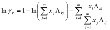
- Using nonlinear regression and a standard sum of squared residuals objective function, use the activity coefficients computed from the raw data to regress the 6 constants for the ternary Wilson equation (below), for this system. Assess the quality of the fit by graphical methods and computing the average percent relative deviations (APRD), which are average fit errors x 100.
- Converge on the true optimal values from several different directions in response parameter space by using a factorial method for the initial guesses. Compute the precision of the GC measurements by sufficiently replicating one GC sample to determine relative precisions according to the t-statistic, and use the precisions to determine whether to accept / reject a particular GC measurement by appropriate hypothesis test.
- Compare the relative precisions of the GC measurement to the APRDs, and discuss. Also report the absolute precisions of the pressure and temperature gauges – determine these once per day.
Understanding the distribution of chemical components in both the vapor and liquid phase, called vapor-liquid equilibrium is essential to the design, operation, and analysis of many engineering processes. Vapor-liquid equilibrium or VLE is a state at which a pure component or mixture exists in both the liquid and vapor phases. The phases are at equilibrium meaning that there were no changes in the macroscopic properties of the system over time. Single component VLE is simple to visualize. Take for example water which is at equilibrium in the vapor and liquid phase at 100 degrees Celsius and one atm. Above this temperature water is a vapor. Below it, water is a liquid. However, engineers generally encounter processes with mixtures in equilibrium making the analysis of VLE more complex and therefore essential to process design. This video will illustrate the principles behind vapor-liquid equilibrium of mixtures and demonstrate how to analyze the VLE of a mixture in the laboratory. Finally, some applications of VLE in the chemical engineering field will be introduced.
When a heated mixture is in a vapor-liquid equilibrium, the vapor and liquid phases generally do not have the same composition. The substance with the lower boiling point will have a higher concentration in the vapor than the substance with the higher boiling point. Thus, engineers refer to components in each phase by their mole fraction where xi is the mole fraction of species i in the liquid and yi is the mole fraction of species i in the vapor phase. This relationship is often depicted using an xy curve like the one shown here for a mixture of two components which illustrates the relationship between each component in each phase. A starting point for all VLE calculations is the simple equilibrium criterion where the fugacity of the species in the vapor equals the fugacity of the species in the liquid. Fugacity is a property related to the exponential difference between the real and ideal gas Gibbs energies. The vapor phase fugacity is equal to the mole fraction of species i in the vapor phase times the pure component vapor fugacity. The expression can be simplified as the pure component vapor fugacity is approximately equal to pressure at low pressure. Liquid phase fugacities are expressed in terms of an activity coefficient, gamma. The activity coefficient is defined as the ratio of a component’s fugacity in an actual mixture to the fugacity of an ideal solution of the same composition. At the saturation vapor pressure the pure component liquid fugacity would equal the saturation vapor pressure because the pure vapor and liquid are in equilibrium there. Finally, since the liquid and vapor fugacities are equal, we can further simplify the relationship as shown which is also known as Raoult’s law. The saturation vapor pressure is often calculated using the Antoine equation where the constants A, B, and C are species-specific and can be found in the literature. Thus, if we measure the compositions of the vapor and liquid which are in equilibrium, we can directly calculate the activity coefficients by measuring temperature and pressure and therefore the saturation vapor pressure. In this experiment a ternary mixture of methanol, isopropyl alcohol and water will be investigated. Various compositions of the mixture are boiled in a VLE apparatus and the lower boiling point components vaporize and are collected in a separate container while the liquid gathers back into the initial sample vessel. Once equilibrium is reached, the liquid and condensed vapor fractions are collected and analyzed with gas chromatography. Using temperature and the liquid and vapor mole fractions the activity coefficients can be calculated. Now that you’ve been introduced to the concepts of VLE and the testing apparatus, let’s see how to carry out the experiment in the laboratory.
To start, drain any liquid out of the system into a waste flask. Keep in mind that the liquid may not completely drain. For the first run add a mixture of 50% methanol, 30% IPA and 20% water through the opening at the top. After filling the mixture, turn on the heater power and condenser water. The apparatus will require roughly 20 minutes to approach equilibrium. The system is now ready to begin the experiment.
When the sample begins boiling, release the stopper to vent the inert outlet of the system. Condensed vapor will start collecting. When equilibrium is reached, steady drips of condensed vapor and returns liquid should be observed. With the temperature stable to within 0.3 degrees for 10 minutes, collect about 1/2 milliliter of liquid in sample vials from both the condensed vapor and the boiling liquid. Drain the condensed vapor from the last sample. Then add a new sample consisting of either 20 milliliters of pure methanol or 50-50 methanol-isopropanol through the sample port. This will give a new overall composition. Reestablish the equilibrium as performed before, however expect a temperature difference from the previous sample. Repeat the equilibration and sampling procedure as before, and then collect the sample to be analyzed. Continue the experiment using different mixtures of the three components. 12 points are sufficient to determine the activity coefficients and the binary interaction coefficients. When all the mixtures have been run, shut down the system by turning off the heaters. When the apparatus begins to cool, shut off the condenser water. Finally measure the composition of each liquid and vapor sample with the gas chromatograph or GC.
Using the system temperature and the liquid and vapor mole fractions acquired from GC, calculate the activity coefficients. This first requires that the saturation pressure is calculated using the Antoine equation where the constants A, B and C for each component can be found in the literature. Now we can use the calculated activity coefficients to correlate the data to a model. We will use the Wilson equation for a ternary mixture which accounts for deviations from ideality in a mixture. The nine lambda constants are the Wilson constants which equal one when i equals j. For each ij pair, there are two different constants. Use a nonlinear regression and a standard sum of squares residual function to determine the six remaining Wilson constants using the mole fraction data from the experiment. The Wilson constants are then used to determine the expected activity coefficients for each component of each sample. Here we show the modeled activity coefficient plotted against the experimental activity coefficients. Ideally, the modeled and experimental activity coefficients would fall along the y equals x line. As you can see in general, the modeled and experimental values fit along this line showing that the model is a good fit to the real system.
Understanding and manipulating the vapor-liquid equilibrium of mixtures is a vital component to a range of processes especially separations. Distillation columns separate mixtures based on their volatility with different compositions of each component in the liquid and vapor phrases on each tray. The more volatile component is vaporized and collected at the top of the column, while the less volatile component remains liquid and is collected at the bottom. VLE data of the components of the mixture is used to determine the number of trays needed to achieve separation in a distillation column. This helps engineers optimize the separation process while keeping operating costs low. Another valuable separation technique using VLE is flash separation. Flash separation is based on the fact that a liquid at a pressure equal to or greater than its bubble point pressure flashes meaning that it partially evaporates when the pressure is reduced. The feed is preheated thus consisting of some liquid and some vapor in equilibrium. It then flows through a pressure reducing valve into the separator. The degree of vaporization and therefore the amount of the solute in the vapor or liquid phases depends on the initial state of the feed stream.
You’ve just watched Jove’s introduction to vapor-liquid equilibrium. You should now understand the concepts behind VLE, how it’s measured in the laboratory, and some of its uses in engineering processes. Thanks for watching.
The activity coefficients of the data do not show significant deviations from a mean value for each component (Table 1). This is as expected because for intermediate component compositions there are not large variations. However, components near 1 have γ's near 1. Low composition components have high γ's. Components highest in concentration in a mixture which will have a reduced deviation, therefore it will be closer to ideal (γ = 1). Components with lower concentrations in a mixture will have higher deviations, so their γ's will be greater than 1.

Table 1: Results of each sampling of the experimental data.
The data were fit to Wilson model parameters and the coefficients were calculated (Table 2). A simple reduction in the sum of squared residuals between experimental and Wilson equation (1) activity coefficients was used. This was achieved using Excel's solver function. The parity plot shown relates the Wilson's Equation model activity coefficients to the experimentally found activity coefficients. The experimental activity coefficients were calculated and graphically compared to the calculated model coefficients.

Table 2: Results of fitting the data to the Wilson model parameters.
(1)
The parameter values found were the best fit (Table 3). Ideally the correlation is along the y=x line; however, a significant correlation resembling the ideal scenario was found (Figure 2). The activity coefficients of the data did not show significant deviations from a mean value for each component, as expected. A reduction in the sum of squared residuals between experimental and Wilson equation activity coefficients was used with Excel's solver function. The parity plot relates the Wilson's Equation model activity coefficients to the experimentally found activity coefficients.

Table 3: Model parameters with water (a), MeOH (b), and IPA (c). The experimental values are compared to expected values.
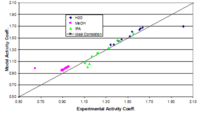
Figure 2: Depiction of the correlation between the experimental activity coefficients and the model activity coefficients.