Starting from the original “fluid mosaic” model by Singer and Nicolson, the picture of cellular plasma membrane has been continuously updated during the last decades in order to include the emerging role of cytoskeleton and lipid domains1,2.
The first observations were obtained by fluorescent recovery after photobleaching (FRAP) unveiling that a significant fraction of membrane proteins is immobile3-5. These pioneering studies, although very informative, suffered from the relatively poor resolution in space (microns) and time (seconds) of FRAP setups. Also, being an ensemble averaging measurement, FRAP lacks in giving information on single molecule behavior.
In this context, the possibility to specifically label a single molecule with very bright tags (allowing the study of the diffusion process one molecule at a time) has been very successful. Particularly, by pushing the time resolution of the Single Particle Tracking (SPT) approach to the microseconds timescale, Kusumi, et al. gained access to unknown features of lipid and protein dynamics that greatly contributed to the recognition of the role of actin-based membrane skeleton in membrane physiology6,7. These findings generated the so-called the ‘picket and fence’ model, in which lipid and protein diffusion is regulated by actin-based skeleton. However, in order to have access to the huge amount of information provided by SPT many experimental issues have to be addressed. Particularly, the labeling procedure is typically composed by many steps like production, purification and introduction of the labeled species into the system. Furthermore, big labels, like quantum dots or metal nanoparticles, are often required to reach the sub-millisecond timescale and the crosslinking of the target molecules by the label could not be avoided in many cases. Finally, many trajectories have to be recorded to fit statistical criteria and concomitantly a low-density of the label is required to allow tracking.
Compared to SPT, fluorescence correlation spectroscopy (FCS), overcoming many of these drawbacks, represents a very promising approach to study molecular dynamics. In fact, FCS works well also with dim and dense labels, enabling to study the dynamics of fluorescent protein-tagged molecules in transiently transfected cells. Also, it allows reaching high statistics in a limited amount of time. Finally, despite the “high” density of labels FCS provides single molecules information. Thanks to all these properties, FCS represents a very straightforward approach and has been extensively applied to study lipid and protein dynamics both in model membranes and in live-cells8-10. Many different approaches have been proposed to increase the ability of FCS to reveal the details of molecular diffusion. For instance, it was shown that by performing FCS on differently-sized observation areas one can define an “FCS diffusion law” enlightening hidden features of molecular motion11,12. Besides being varied in size, the focal area was also duplicated13, moved in space along lines14-20 or conjugated with fast cameras21,22. Using these ‘spatio-temporal’ correlation approaches, relevant biological parameters of several membrane components were quantitatively described on both model membranes and actual biological ones, thus yielding insight into membrane spatial organization.
However, in all the FRAP and FCS applications described so far the size of the focal area represents a limit in spatial resolution that cannot be overcome. Several super-resolution imaging methods have been recently developed to bypass this limit. Some are based on localization precision, such as stochastic optical reconstruction microscopy (STORM)23,24, photoactivation localization microscopy (PALM)25, fluorescence PALM (FPALM)26, and single-particle tracking PALM (sptPALM)27: the relatively large amount of photons required at each snapshot, however, limits the time resolution of these methods to at least several milliseconds, thus hampering their applicability in vivo.
In contrast, a promising alternative for super resolution imaging have been opened by spatially modulating the fluorescence emission with stimulated emission depletion methods (STED or reversible saturable optical fluorescence transitions (RESOLFT))28,29. These approaches combine the shaping of the observation volume well below the diffraction limit with the possibility to use fast scanning microscopes and detection systems. In combination with fluorescence fluctuation analysis, STED microscopy allowed to directly probe the nanoscale spatiotemporal dynamics of lipids and proteins in live cell membranes30,31.
The same physical quantities of STED-based microscopy can be obtained by a modified spatio-temporal image correlation spectroscopy (STICS32,33) method that is suitable for the study of the dynamics of fluorescently-tagged membrane proteins and/or lipids in live cells and by a commercial microscope. The experimental protocol presented here is composed by few steps. The first one requires a fast imaging of the region of interest on the membrane. Then, the resulting stack of images is used to calculate the average spatial-temporal correlation functions. By fitting the series of correlation functions, the molecular ‘diffusion law’ can be obtained directly from imaging in the form of an apparent diffusivity (Dapp)-vs-average displacement plot. This plot critically depends on the environment explored by the molecules and allows recognizing directly the actual diffusion modes of the lipid/protein of interest.
In more details, as previously shown34, the spatio-temporal auto-correlation function of the acquired image series critically depends on the dynamics of the molecules moving in the collected image series (please note that the same reasoning can be applied in a line acquisition where just one dimension in space is considered). In particular, we define the correlation function as:
 (1)
(1)
where  represents the measured fluorescence intensity in the position x, y and at time t,
 ![]() and
and ![]() represents the distance in the x and y directions respectively,
represents the distance in the x and y directions respectively,![]() represents the time lag, and
represents the time lag, and ![]() represents the average. This function can be expressed as:
represents the average. This function can be expressed as:
 (2)
(2)
where ‘N’ represents the average number of molecules in the observation area, ![]() represents the convolution operation in space, and
represents the convolution operation in space, and  represents the autocorrelation of the instrumental waist. This latter can be interpreted as a measure of how the photons of a single emitter are spread out in space due to the optical/recording setup (the so called Point Spread Function, PSF, generally well approximated by a Gaussian function). Finally,
  represents the probability to find a particle at a distance
 ![]() and
and ![]() after a time delay
after a time delay ![]() . If we consider a diffusive dynamics, in which particles move randomly in all directions and net fluxes are not present, this function is also well approximated by a Gaussian function where the variance can be identified as the Mean Square Displacement (MSD) of the moving particle. Thus, the waist of the correlation function (also referred as
. If we consider a diffusive dynamics, in which particles move randomly in all directions and net fluxes are not present, this function is also well approximated by a Gaussian function where the variance can be identified as the Mean Square Displacement (MSD) of the moving particle. Thus, the waist of the correlation function (also referred as ![]() ), can be defined as the sum of the particle MSDs and the instrumental waist and can be measured by a Gaussian fitting of the correlation function for each time delay. The measured iMSD can be used to calculate an apparent diffusivity of the moving molecules
), can be defined as the sum of the particle MSDs and the instrumental waist and can be measured by a Gaussian fitting of the correlation function for each time delay. The measured iMSD can be used to calculate an apparent diffusivity of the moving molecules ![]() and an average displacement
and an average displacement![]() as:
as:
 (3)
(3)
 (4)
(4)
Few considerations on the experimental setup used can guide the reader throughout the following sections. In order to selectively excite the fluorophores on the basal membrane of living cells we will use a total internal reflection (TIR) illumination, using a commercial TIR fluorescence (TIRF) microscope (details can be found in the material section). Moreover, in order to collect the fluorescence we will use a high magnification objective (100X NA 1.47, high numerical aperture is required for TIRF illumination) and an EMCCD camera (physical size of the pixel on the chip 16 μm). To reach a pixel size of 100 nm we apply an additional magnification lens of 1.6X. As discussed below, a time resolution below 1 msec would be required to properly describe the dynamics of fast membrane lipids below 100 nm. In order to reach this temporal resolution we need to select a region of interest (ROI) smaller than the whole chip of the camera (512 x 512). In this way, the camera will read a reduced number of lines increasing the time resolution. However, in this readout regime the frame time would be limited by the time required to shift the charges from the exposure to the readout chip on the camera and is usually in the order of milliseconds for 512 x 512 pixel EMCCD. To beat this limit, an emerging technology allows shifting the ROI-lines only instead of the whole frame, with a practical effective reduction of the exposed chip size (called Cropped Sensor Mode in our EMCCD). For this configuration to be effective, the chip outside of the ROI must be covered by a couple of slits mounted in the optical path. Thanks to this setup a time resolution down to 10-4 seconds can be achieved. Please note, however, that this approach can be coupled with many different experimental setups, as explained in the ‘discussion’ section.
Demonstration of the method will be provided in live cells, by using both an ATTO488 labeled 1-palmitoyl-2-hydroxy-sn-glycero-3-phosphoethanolamine (ATTO488-PPE) and a GFP-labeled variant of the Transferrin Receptor (GFP-TfR). In the case of ATTO488-PPE this approach can successfully recover an almost constant Dapp as a function of average displacement indicating a mostly free diffusion, as previously reported30,35. By contrast, TfR-GFP shows a decreasing Dapp as a function of average displacement, suggesting partially-confined diffusion6. Moreover, in the latter case it is possible to quantify the local diffusion constant and the average confinement area over many microns on the membrane plane.
In order to calibrate the instrumental waist, the image of a single fluorescent nano-bead can be measure as described in Protocol step 1.1. A typical fluorescent image of these beads is presented in Figure 1. The fitting of intensity distribution by a 2D Gaussian function gives back good residuals and allows measuring the instrumental waist at 270 nm. This value is in good agreement with the expected diffraction limit estimated by the Rayleigh equation. This calibration is not necessary for the measurement of particle dynamics but it is required to measure the apparent particle size.
A typical frequency distribution of camera background is presented in Figure 2. The peak at about 180 DL is due to the camera response to no photon, and it represents the contribution of Analog Digital (AD) converter. This contribution can be approximated as a Gaussian distribution to estimate the offset and the variance introduced by the signal recording. Above 200 DL the digital level distribution becomes exponential (linear in logarithmic scale) and represents the average camera response to a single photon. Fitting this part with an exponential distribution allows the measurements of the average DL assigned to each single photon. The higher is the ratio between the average DL assigned to each photon and the AD converter error, the lower will be the noise in the calculated correlation function. Moreover, the average single photon response allows the estimation of the camera dynamic range.
A diagram of the complete experimental procedure is summarized in Figure 3 and a picture of Atto488-PPE insertion into the membrane is represented in Figure 4A. A representative TIRF image of the basal membrane of a CHO cells labeled with Atto488-PPE is presented in Figure 4B. Several bright spots may be present outside the cell due to liposomes stacked on the glass. They can be discarded by selecting a ROI on a membrane portion mostly uniform in fluorescence (i.e., the cellular plasma membrane). As expected the measured diffusion law (Figure 4C) for this lipid is flat, indicating a mostly free diffusion as previously shown by STED-FCS measurements30,35. It is worth mentioning that all the shown displacement values are below the diffraction limit, clearly indicating the ability of this approach to super-resolve average molecular displacements well below the diffraction limit and down to few tens of nanometers.
A schematization of TfR-GFP dimer insertion into the membrane is represented in Figure 5A. Many studies showed that the cytoplasmic tail of this receptor interacts with the membrane skeleton, which in turn acts as a fence for the receptor mobility12,40. A representative TIRF image of a CHO cell expressing TfR-GFP is presented in Figure 5B. Low fluorescence intensity cells should be preferred, as the membrane is closer to the native condition and the probability of artifacts related to the over-expression is minimized. In addition, the central part of the cell should be avoided, as the effects of out-of-focus fluorescence (from cytoplasm, for instance) may be present. As expected the measured diffusion law (Figure 5C) for TfR-GFP shows a first flat behavior below 100 nm, with an average Dapp of about 0.7 µm2sec-1, followed by consequent rapid decrease in apparent diffusivity down to 0.2 µm2sec-1 (the value typically measured by diffraction-limited FCS12). This result shows that our approach can easily measure the average displacement of GFP labeled proteins with a resolution of few tens of nanometers. Moreover the spatial scale at which Dapp starts to decrease sets the characteristic spatial scale of protein partial confinement by the membrane skeleton at around 120 nm, in keeping with previous estimates6.
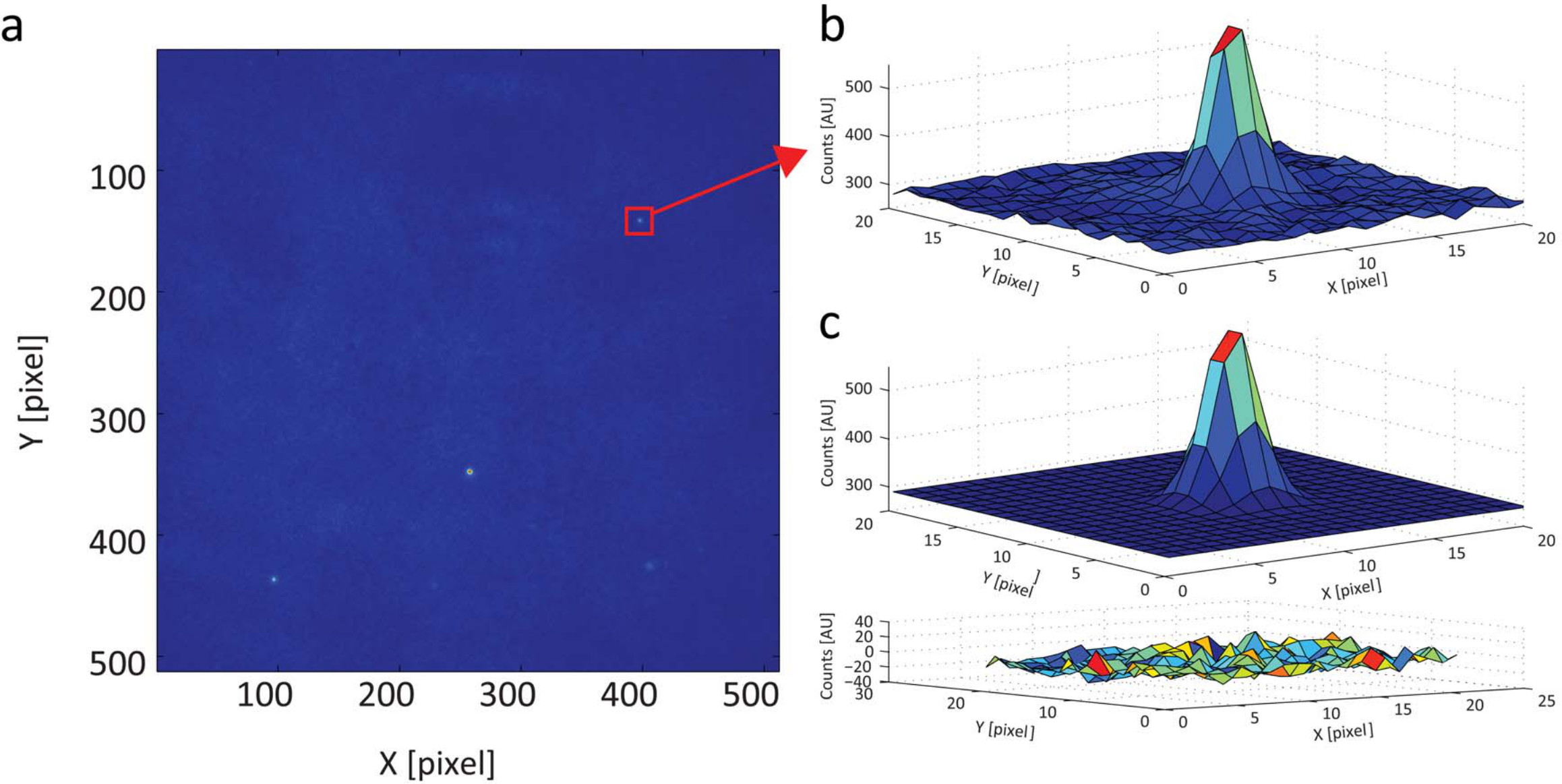
Figure 1. Calibration of Point Spread Function. (A) Pseudocolor image of an isolated bead and beads aggregates. (B) 3D plot of the intensity profile of an isolated bead shows a well-defined Gaussian profile. (C) Fit of the intensity distribution by a Gaussian function (upper panel) with the corresponding residuals (lower panel). The good agreement between the fitted distribution and the measured intensity profile is also a proof that the instrumental PSF can be approximated by a Gaussian function. Please click here to view a larger version of this figure.

Figure 2. Calibration of Camera response to single photons. The figure shows the Digital Level (DL) distribution for camera background in a 32 x 128 ROI, exposure 0.5 msec, in Cropped Sensor Mode. The peak at about 180 DL represents the camera response to no photons. Particularly, it represents the contribution of the Analog Digital (AD) converter and can be approximated by a Gaussian function to estimate the offset and the variance introduced by the signal recording. Above 200 DL the distribution of digital levels becomes exponential and represents the average camera response to a single photon. The measurement of these parameters allows estimating the density of photons that are recorded during the acquisition. Please click here to view a larger version of this figure.

Figure 3. Schematization of the method. (A) Wide field imaging by EMCCD camera is applied to reach sub-millisecond resolution, while TIRF microcopy is exploited to provide accurate optical sectioning of the plasma membrane. (B) The resulting stack of images is autocorrelated in order to calculate the average spatial-temporal correlation function. This correlation function is well approximated by a Gaussian function (see Introduction) and it spreads out in time according to particle displacements. (C) Thus, in order to quantify the spreading of the correlation function due to molecular displacement, fitting with a Gaussian function is performed. This allows measuring the molecular ‘diffusion law’ directly from imaging, in the form of apparent diffusivity vs average displacement plot. (D) Thanks to this plot, molecular diffusion modes can be directly identified with no need for an interpretative model or assumptions about the spatial organization of the membrane. In fact, freely diffusing molecules will display a constant apparent diffusivity as their mobility does not depend on the spatial scale of the measurement. By contrast, partially confined molecules will display a quite constant apparent diffusivity for displacements smaller than confinement size, then a decreasing diffusivity for spatial scales bigger than confinement size. Thus, the appearance of a reduction in the apparent diffusivity can be interpreted as a fingerprint of transient confinement, while the related spatial scale can be used to estimate the spatial extension of the confinement. Please click here to view a larger version of this figure.
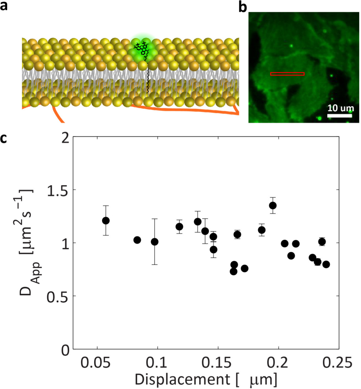
Figure 4. ATTO488-PPE diffusion law in live cell membranes. (A) Schematic representation of ATTO488-PPE insertion in cell membrane. (B) TIRF image of CHO basal membrane labeled with ATTO488-PPE: a ROI (red box) is selected in a mostly uniform part of the cell, avoiding cell border and highly fluorescent spots. (C) The diffusion law measured in the selected ROI shows a flat behavior confirming a free diffusion model for this component. Please click here to view a larger version of this figure.

Figure 5. TfR-GFP diffusion law in live cell membranes. (A) Schematic representation of TfR-GFP insertion in cell membrane: the cytoplasmic tail of the receptor interacts with the membrane skeleton, that acts as a fence for receptor mobility. (B) TIRF image of CHO expressing TfR-GFP: a ROI is selected preferring low expressing cells to avoid artefacts due to overexpression. (C) The diffusion law of TfR (black dots), unlike PPE (gray line, taken from Figure 4), shows the typical behavior of partially confined diffusion where a first flat part is followed by a decrease in Dapp. Please click here to view a larger version of this figure.
