Summary
Mixed-effects models are flexible and useful tools for analyzing data with a hierarchical stochastic structure in forestry and could also be used to significantly improve the performance of forest growth models. Here, a protocol is presented that synthesizes information relating to linear mixed-effects models.
Abstract
Here, we developed an individual-tree model of 5-year basal area increments based on a dataset including 21898 Picea asperata trees from 779 sample plots located in Xinjiang Province, northwest China. To prevent high correlations among observations from the same sampling unit, we developed the model using a linear mixed-effects approach with random plot effect to account for stochastic variability. Various tree- and stand-level variables, such as indices for tree size, competition, and site condition, were included as fixed effects to explain the residual variability. In addition, heteroscedasticity and autocorrelation were described by introducing variance functions and autocorrelation structures. The optimal linear mixed-effects model was determined by several fit statistics: Akaike’s information criterion, Bayesian information criterion, logarithm likelihood, and a likelihood ratio test. The results indicated that significant variables of individual-tree basal area increment were the inverse transformation of diameter at breast height, the basal area of trees larger than the subject tree, the number of trees per hectare, and elevation. Furthermore, errors in variance structure were most successfully modeled by the exponential function, and the autocorrelation was significantly corrected by first-order autoregressive structure (AR(1)). The performance of the linear mixed-effects model was significantly improved relative to the model using ordinary least squares regression.
Introduction
Compared with even-aged monoculture, uneven-aged mixed-species forest management with multiple objectives has received increased attention recently1,2,3. Prediction of different management alternatives is necessary for formulating robust forest management strategies, especially for complex uneven-aged mixed-species forest4. Forest growth and yield models have been used extensively to forecast tree or stand development and harvest under various management schemes5,6,7. Forest growth and yield models are classified into individual-tree models, size-class models, and whole-stand growth models6,7,8. Unfortunately, size-class models and whole-stand models are not appropriate for uneven-aged mixed-species forests, which require a more detailed description to support the forest management decision-making process. For this reason, individual-tree growth and yield models have received increased attention throughout the last few decades because of their ability to make predictions for forest stands with a variety of species compositions, structures, and management strategies9,10,11.
Ordinary least squares (OLS) regression is the most commonly used method for the development of individual-tree growth models12,13,14,15. The datasets for individual-tree growth models collected repeatedly over a fixed length of time on the same sampling unit (i.e., sample plot or tree) have a hierarchical stochastic structure, with a lack of independence and high spatial and temporal correlation among observations10,16. The hierarchical stochastic structure violates the fundamental assumptions of OLS regression: namely independent residuals and normally distributed data with equal variances. Therefore, the use of OLS regression inevitably produces biased estimates of the standard error of parameter estimates for these data13,14.
Mixed-effects models provide a powerful tool for analyzing data with complex structures, such as repeated measures data, longitudinal data, and multi-level data. Mixed-effects models consist of both fixed components, common to the complete population, and random components, which is specific to each sampling level. In addition, mixed-effects models take into account heteroscedasticity and autocorrelation in space and time by defining non-diagonal variance-covariance structure matrices17,18,19. For this reason, mixed-effects models have been extensively used in forestry, such as in diameter-height models20,21, crown models22,23, self-thinning models24,25, and growth models26,27.
Here, the main objective was to develop an individual-tree basal area increment model using a linear mixed-effects approach. We hope that the mixed-effects approach could be broadly applied.
Subscription Required. Please recommend JoVE to your librarian.
Protocol
1. Data preparation
- Prepare modeling data, which includes individual-tree information (species and diameter at breast height at 1.3 m) and plot information (slope, aspect, and elevation). In this study, the data were obtained from the 8th (2009) and 9th (2014) Chinese National Forest Inventory in Xinjiang Province, northwest China, which includes 21,898 observations of 779 sample plots. These sample plots are square-shaped with a size of 1 Mu (Chinese unit of area equivalent to 0.067 ha) and are systematically arranged over a grid of 4 km x 8 km.
NOTE: Data for modeling (basal area) increment requires at least one growth period (i.e., two observations). - Randomly divide the data into two datasets, with 80% of the data from the sample plots used for model fitting (model development dataset), which consists of 17,145 observations from 623 sample plots and 20% for model validation (model validation dataset) which consists of 4,753 observations from 156 sample plots. Descriptive statistics for the key variables used are provided in Table 1.
NOTE: This step of the modeling procedure can be omitted, and all data is used for model development.
| Variables | Fitting data | Validation data | |||||||
| Min | Max | Mean | S.D. | Min | Max | Mean | S.D. | ||
| DBH1 (cm) | 5 | 124.8 | 19.9 | 13.2 | 5 | 101.5 | 19.5 | 13.4 | |
| QMD (cm) | 6.7 | 82.3 | 22.5 | 8.5 | 9.2 | 73.3 | 21.8 | 9.2 | |
| ID (cm) | 0.1 | 14.4 | 1.1 | 1 | 0.1 | 16.9 | 1 | 1.1 | |
| BAL (m3) | 0 | 5.2 | 1.7 | 0.9 | 0 | 5.4 | 1.7 | 1 | |
| NT (trees/ha) | 14.9 | 3642 | 1072 | 673.7 | 14.9 | 3418 | 1205 | 829.3 | |
| BA (m2/ha) | 0.1 | 77.5 | 34.2 | 13.9 | 0.1 | 80.6 | 34.5 | 15.3 | |
| EL (m) | 2 | 3302 | 2189 | 340.3 | 1441 | 3380 | 2256 | 308.3 | |
Table 1. Summary statistics for fitting and validation data. DBH1: initial diameter at breast height at 1.3 m (DBH), DBH2: DBH measured after 5 years of growth, QMD: quadratic mean diameter, ID: diameter increment for 5 years (DBH2 – DBH1), BAL: the basal area of trees larger than the subject tree (the subject tree: the tree which was calculated the competition indices), NT: the number of trees per hectare, BA: basal area per hectare, EL: elevation, S.D.: standard deviation.
2. Basic model development
- Consult references to identify variables that affect individual-tree basal area increments.
- Select and compute variables based on the data. Generally, the individual-tree basal area increment is affected by three groups of variables: tree size, competition, and site condition27,28,29,30.
- Consider tree-size effects such as DBH1, square of DBH1 (
 ), the inverse transformation of DBH1 (1/DBH1), and the common logarithm of DBH1 (logDBH1) or combinations of them.
 - Consider competitive effects such as both one- and two-sided indices of competition to more comprehensively quantify the level of competition experienced by a tree, as well as its social position within the stand. One-sided competition include BAL and the relative density index (RD=DBH1/QMD); two-sided competition include NT, and BA.
NOTE: The distance dependent competition indices should be considered if data is available. - Consider site effects such as aspect (ASP), slope (SL), and EL. SL and ASP should be included using Stage’s transformation31.
- Consider tree-size effects such as DBH1, square of DBH1 (
- Select log(
 - +1) ( denotes square of DBH2) as the dependent variable.
 - Develop the basic model using the stepwise regression method. Ensure that the model is biologically reasonable and exhibits significant differences between independent variables. Utilize the variance inflation factor (VIF) to check for multicollinearity.
- Leave the independent variables with p < 0.05 and VIF < 5 in the basic model.
- Output the basic model results and the residual plot. The basic model produced here serves as a foundation for the further development of a mixed-effects model.
 ), the inverse transformation of DBH1 (1/DBH1), and the common logarithm of DBH1 (logDBH1) or combinations of them.
 -
- 3. Linear mixed-effects model development with the package “nlme” in R software
- Read the model development dataset and load the Package “nlme”.
>model.development.dataset=read.csv("E:/DATA/JoVE/modelingdata.csv",
header=TRUE)
>library(nlme) - Select sample plots as random effects to develop the mixed-effects model.
- Fit all possible combinations of random effects with the maximum likelihood (ML) method and output the results.
>Model<-lme(Y~1/DBH1+BAL+NT+EL,data=model.development.dataset,
method="ML", random =~1|PLOT)
>summary(Model)- Set random =~1 is the intercept to random parameters. Change the random statements until all combinations are fitted. For example, to set 1/DBH1 and BAL as random parameters, the code is as follows: random =~1/DBH1+BAL-1. In addition, in the process of fitting, the codes may report errors due to the nonconvergence of the fitted model.
- Select the best model by Akaike’s information criterion (AIC), the Bayesian information criterion (BIC), the logarithm likelihood (Loglik), and likelihood ratio test (LRT).
>anova(Model.1, Model.6)
>anova(Model.6, Model.23)
>anova(Model.23, Model.30) - Determine the structure of Ri. Address the heteroscedasticity and autocorrelation of Ri32. The Ri is written as follows:
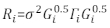 (1)
(1)
where σ2 is an unknown scaling factor that is equal to the model residual variance, Gi is a diagonal matrix describing heteroscedasticity, and Γi is a matrix describing autocorrelation.- Observe whether the residuals have heteroscedasticity from the residual plot. If there is heteroscedasticity (the residuals have a clear pattern or trend), introduce three frequently used variance functions—the constant plus power function, the power function, and the exponential function—to model the errors variance structure.
>Model.30.1<-lme(Y~1/DBH1+BAL+NT+EL,data=model.development.dataset, method="ML",random=~1/DBH1+BAL+NT|PLOT,
weights=varConstPower(form=~ fitted(.)))
>summary(Model.30.1)
>Model.30.2<-lme(Y~1/DBH1+BAL+NT+EL,data=model.development.dataset, method="ML",random=~1/DBH1+BAL+NT|PLOT,
weights=varPower(form=~ fitted(.)))
>summary(Model.30.2)
>Model.30.3<-lme(Y~1/DBH1+BAL+NT+EL,data=model.development.dataset, method="ML",random=~1/DBH1+BAL+NT|PLOT,
weights=varExp(form=~ fitted(.)))
>summary(Model.30.3) - Determine the best variance function for the model according to the AIC, BIC, Loglik, and LRT.
>anova(Model.30, Model.30.1)
>anova(Model.30, Model.30.2)
>anova(Model.30, Model.30.3) - Introduce three commonly used autocorrelation structures—the compound symmetry structure (CS), first-order autoregressive structure [AR(1)], and a combination of first-order autoregressive and moving average structures [ARMA(1,1)]—to account for autocorrelation.
>Model.30.3.1<-lme(Y~1/DBH1+BAL+NT+EL,data=model.development.dataset, method="ML",
random=~1/DBH1+BAL+NT|PLOT, weights=varExp(form=~fitted(.)), corr= corCompSymm())
>summary(Model.30.3.1)
>Model.30.3.2<-lme(Y~1/DBH1+BAL+NT+EL,data=model.development.dataset, method="ML",
random=~1/DBH1+BAL+NT|PLOT,weights=varExp(form=~ fitted(.)), corr=corAR1())
>summary(Model.30.3.2)
>Model.30.3.3<-lme(Y~1/DBH1+BAL+NT+EL,data=model.development.dataset, method="ML",
random=~1/DBH1+BAL+NT|PLOT,weights=varExp(form=~ fitted(.)), corr=corARMA(q=1,p=1))
>summary(Model.30.3.3) - Determine the best autocorrelation structure according to the AIC, BIC, Loglik, and LRT.
>anova(Model.30.3, Model.30.3.2)
NOTE: The Gi and Γi cannot be defined if there is no heteroscedasticity and autocorrelation. - Output the final results of the mixed-effects model using the restricted maximum likelihood (REML) method.
>Mixed.model<-lme(Y~1/DBH1+BAL+NT+EL,data=model.development.dataset, method="REML",random=~1/DBH1+BAL+NT|PLOT,
weights=varExp(form=~ fitted(.)), corr=corAR1())
>summary(Mixed.model)
- Observe whether the residuals have heteroscedasticity from the residual plot. If there is heteroscedasticity (the residuals have a clear pattern or trend), introduce three frequently used variance functions—the constant plus power function, the power function, and the exponential function—to model the errors variance structure.
 (1)
(1)4. Bias correction
- Transform the predicted values of basal area increment using the final model on a logarithmic scale to the original scale. However, such a linear back transformation of predicted value from a log-transformed model produces an associated log-transformation bias. To deal with the log-bias, a correction factor was derived and integrated into the prediction equation, which estimates actual predicted basal area increment for a given tree [Equation (2)]:
 (2)
(2)
where is predicted logarithmic value of basal area increment from the model, while
  is the predicted back transformed value of basal area increment for 5 years after correcting for log-transformation bias.
  is variance from random effects at plot and σ2 is residual variance.
 - Convert basal area increment ( ) to the diameter increment.
 (2)
(2) is predicted logarithmic value of basal area increment from the model, while
  is the predicted back transformed value of basal area increment for 5 years after correcting for log-transformation bias.
  is variance from random effects at plot and σ2 is residual variance.
5. Model prediction and evaluation
- Prepare the model validation dataset produced in section 1.2 for prediction.
- Use the linear mixed-effects model to predict individual-tree basal area increment. The random components were calculated using the following best linear unbiased predictor:
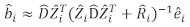 (3)
(3)
where is a vector for the random components;
  is the variance-covariance matrix for between-plots variability;
  is the design matrix for the random components acting at the complementary observations;
  is the residual vector whose components are given by the difference between the basal area increments and the predicted increments using the fixed-effects model.
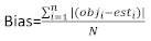
 - Evaluate and compare the predictive ability of the basic model and the linear mixed-effects model using the following three statistical indicators23,33.
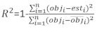 (4)
(4)
 (5)
(5)
 (6)
(6)
where obji is the basal area increments, esti is the predicted basal area increments, is the mean of observations, and N is the number of observations.
 (3)
(3) is a vector for the random components;
  is the variance-covariance matrix for between-plots variability;
  is the design matrix for the random components acting at the complementary observations;
  is the residual vector whose components are given by the difference between the basal area increments and the predicted increments using the fixed-effects model.
 (4)
(4) (5)
(5) (6)
(6) is the mean of observations, and N is the number of observations.
Subscription Required. Please recommend JoVE to your librarian.
Representative Results
The basic basal area increment model for P. asperata was expressed as Equation (7). The parameter estimates, their corresponding standard errors, and the lack-of-fit statistics are shown in Table 2. The residual plot is shown in Figure 1. Pronounced heteroscedasticity of the residuals was observed.
 (7)
(7)
| Estimate | Standard error | t-test | P-value | VIF | |
| int | 2.41 | 2.26E-02 | 106.78 | <2e-16 | - |
| 1/DBH1 | -5.84 | 7.57E-02 | -77.19 | <2e-16 | 1.12 |
| BAL | -0.0954 | 3.34E-03 | -28.54 | <2e-16 | 1.08 |
| NT | -0.000158 | 4.74E-06 | -33.31 | <2e-16 | 1.12 |
| EL | -0.00011 | 9.07E-06 | -12.13 | <2e-16 | 1.05 |
| AIC = 16789 | |||||
| BIC = 16836 | |||||
| Loglik = -8389 | |||||
Table 2. Basic model results. The estimated parameters, their corresponding standard errors, and the lack-of-fit statistics derived from Equation (7). VIF: variance inflation factor, AIC: Akaike’s information criterion, BIC: Bayesian information criterion, and Loglik: logarithm likelihood.

Figure 1. Residual plot derived from Equation (7). The residuals have a clear trend, i.e., pronounced heteroscedasticity of the residuals was observed. Please click here to view a larger version of this figure.
There were 31 possible combinations of random-effects parameters for Equation (7). After fitting, 30 combinations reached convergence (Table 3). Among these 30 combinations, Model 30 of Equation (8) was selected since it yielded the lowest AIC (9083), the lowest BIC (9207), the largest LogLik (-4525), and the LRT was significantly different when compared with the other models.
 (8)
(8)
where β1 – β5 are the fixed effects parameters and b1 – b4 are the random-effects parameters.
| Model | Random parameters | AIC | BIC | LogLik | LRT | P-value | ||||
| int | 1/DBH1 | BAL | NT | EL | ||||||
| 1 | ▲ | 10175 | 10230 | -5081 | ||||||
| 2 | ▲ | 11630 | 11684 | -5808 | ||||||
| 3 | ▲ | 11772 | 11826 | -5879 | ||||||
| 4 | ▲ | 10556 | 10611 | -5271 | ||||||
| 5 | ▲ | 10259 | 10313 | -5123 | ||||||
| 6 | ▲ | ▲ | 9268 | 9338 | -4625 | 911.1 | <.0001 | |||
| (1 vs 6) | ||||||||||
| 7 | ▲ | ▲ | 9411 | 9481 | -4697 | |||||
| 8 | ▲ | ▲ | 10179 | 10249 | -5081 | |||||
| 9 | ▲ | ▲ | 10179 | 10249 | -5080 | |||||
| 10 | ▲ | ▲ | 10829 | 10899 | -5406 | |||||
| 11 | ▲ | ▲ | 9532 | 9601 | -4757 | |||||
| 12 | ▲ | ▲ | 9335 | 9405 | -4659 | |||||
| 13 | ▲ | ▲ | 9803 | 9873 | -4892 | |||||
| 14 | ▲ | ▲ | 9465 | 9535 | -4723 | |||||
| 15 | ▲ | ▲ | 10200 | 10270 | -5091 | |||||
| 16 | ▲ | ▲ | ▲ | Nonconvergence | ||||||
| 17 | ▲ | ▲ | ▲ | 9271 | 9364 | -4624 | ||||
| 18 | ▲ | ▲ | ▲ | 9274 | 9367 | -4625 | ||||
| 19 | ▲ | ▲ | ▲ | 9417 | 9510 | -4696 | ||||
| 20 | ▲ | ▲ | ▲ | 9417 | 9510 | -4697 | ||||
| 21 | ▲ | ▲ | ▲ | 10184 | 10277 | -5080 | ||||
| 22 | ▲ | ▲ | ▲ | 9332 | 9425 | -4654 | ||||
| 23 | ▲ | ▲ | ▲ | 9132 | 9225 | -4554 | 142.7 | <.0001 | ||
| (23 vs 6) | ||||||||||
| 24 | ▲ | ▲ | ▲ | 9293 | 9386 | -4634 | ||||
| 25 | ▲ | ▲ | ▲ | 9443 | 9536 | -4709 | ||||
| 26 | ▲ | ▲ | ▲ | ▲ | 9083 | 9207 | -4525 | |||
| 27 | ▲ | ▲ | ▲ | ▲ | 9086 | 9210 | -4527 | |||
| 28 | ▲ | ▲ | ▲ | ▲ | 9280 | 9404 | -4624 | |||
| 29 | ▲ | ▲ | ▲ | ▲ | 9425 | 9549 | -4696 | |||
| 30 | ▲ | ▲ | ▲ | ▲ | 9083 | 9207 | -4525 | 56.8 | <.0001 | |
| (30 vs 23) | ||||||||||
| 31 | ▲ | ▲ | ▲ | ▲ | ▲ | 9091 | 9254 | -4525 | ||
Table 3. Evaluation indices of each linear mixed-effects model. ▲: random-effects parameter was selected for fitting; LRT: likelihood ratio test.
The linear mixed-effects models with variance functions and correlation structures are shown in Table 4. According to the AIC, BIC, Loglik, and LRT, the exponential function and AR(1) were selected as the best variance function and autocorrelation structure, respectively.
| Model | Variance function | Correlation structure | AIC | BIC | LogLik | LRT | P-value |
| 30 | No | Independent | 9083 | 9207 | -4525 | ||
| 30.1 | ConstPower | Independent | 9075 | 9215 | -4520 | 11.8a | 0.0028 |
| 30.2 | Power | Independent | 9073 | 9205 | -4520 | 11.7a | 6.00E-04 |
| 30.3 | Exponent | Independent | 9073 | 9204 | -4519 | 12.3a | 5.00E-04 |
| 30.3.1 | Exponent | CS | Nonconvergence | ||||
| 30.3.2 | Exponent | AR(1) | 9050 | 9189 | -4507 | 24.9b | <.0001 |
| 30.3.3 | Exponent | ARMA(1,1) | Nonconvergence | ||||
Table 4. Comparisons of the linear mixed-effects individual-tree basal area increment models performance with different variance functions and different correlation structures. CS: compound symmetry structure, AR(1): a first-order autoregressive structure, ARMA(1,1): a combination of first-order autoregressive and moving average structures; a Likelihood ratio was calculated for Model 30; b Likelihood ratio was calculated for Model 30.3.
The final linear mixed-effects individual-tree basal area increment model was proposed using the REML method [Equation (9)]. The estimated fixed parameters, their corresponding standard errors, and the lack-of-fit statistics are shown in Table 5. The residual plot of the final model is shown in Figure 2. A significant improvement was observed in the residuals.
 (9)
(9)
where
 (10)
(10)
| Estimate | Standard error | t-Test | P-value | |
| int | 2.8086 | 7.99E-02 | 35.14 | <0.01 |
| 1/DBH1 | -6.2402 | 1.56E-01 | -40.01 | <0.01 |
| BAL | -0.1324 | 8.07E-03 | -16.41 | <0.01 |
| NT | -0.0001 | 2.26E-05 | -4.921 | <0.01 |
| EL | -0.0003 | 3.32E-05 | -7.86 | <0.01 |
| AIC = 9105 | ||||
| BIC = 9244 | ||||
| Loglik = -4535 | ||||
Table 5. Mixed-effects model results. The estimated fixed parameters, their corresponding standard errors, and the lack-of-fit statistics derived from Equation (9).

Figure 2. Residual plot derived from Equation (9). Compared with Figure 1, a significant improvement was observed in the residuals. Please click here to view a larger version of this figure.
Table 6 listed the three prediction statistics of Equation (7) and Equation (9). Compared with the basic model, the performance of the linear mixed-effects model was significantly improved.
| Model | Bias | RMSE | R2 |
| Basic model | 0.297 | 0.377 | 0.479 |
| Mixed-effects model | 0.221 | 0.286 | 0.699 |
Table 6. Evaluation indices of the basic model and the linear mixed-effects model. A significant improvement was observed from the three prediction statistics.
Subscription Required. Please recommend JoVE to your librarian.
Discussion
A crucial issue for the development of mixed-effects models is to determine which parameters can be treated as random effects and which should be considered fixed effects34,35. Two methods have been proposed. The most common approach is to treat all parameters as random effects and then have the best model selected by AIC, BIC, Loglik, and LRT. This was the method employed by our study35. An alternative is to fit basal area increment models for every sample plot with OLS regression. Parameters that have high variability and less overlap in confidence intervals across the sample plots among these models can be regarded as random ones17.
To account for heteroscedasticity and autocorrelation, three variance functions and three autocorrelation structures were introduced. Consistent with the results of Calama and Montero17 and Uzoh and Oliver27, the exponential function and AR(1) were determined to be the optimal variance function and autocorrelation structure, respectively.
There are two most commonly used methods in statistical software programs to estimate mixed-effects models: ML and REML17. ML is more flexible because models that differ in either their fixed effects or their random effects can be directly compared. However, the estimator for the variance obtained by ML is biased because ML does not account for the fact that the intercept and slope are estimated as well (as opposed to being known for certain). REML can provide superior ML estimates. Therefore, when the model comparisons were completed, the REML method was used for final model fitting17,18,36.
In this study, we found that the individual-tree basal area increment model for P. asperata using a linear mixed-effects approach represented a significant improvement over the basic model using OLS regression. Mixed-effects models provide an efficient tool for modeling data with hierarchical stochastic structure, making it widely applicable in fields such as agriculture, biology, economics, manufacturing, and geophysics.
Subscription Required. Please recommend JoVE to your librarian.
Disclosures
The authors have nothing to disclose.
Acknowledgments
This research was funded by the Fundamental Research Funds for the Central Universities, grant number 2019GJZL04. We thank Professor Weisheng Zeng at the Academy of Forest Inventory and Planning, National Forestry and Grassland Administration, China for providing access to data.
Materials
| Name | Company | Catalog Number | Comments |
| Computer | acer | ||
| Microsoft Office 2013 | |||
| R x64 3.5.1 |
References
- Meng, J., Lu, Y., Ji, Z. Transformation of a Degraded Pinus massoniana Plantation into a Mixed-Species Irregular Forest: Impacts on Stand Structure and Growth in Southern China. Forests. 5 (12), 3199-3221 (2014).
- Sharma, A., Bohn, K., Jose, S., Cropper, W. P. Converting even-aged plantations to uneven-aged stand conditions: A simulation analysis of silvicultural regimes with slash pine (Pinus elliottii Engelm). Forest Science. 60 (5), 893-906 (2014).
- Zhu, J., et al. Feasibility of implementing thinning in even-aged Larix olgensis plantations to develop uneven-aged larch–broadleaved mixed forests. Journal of Forest Research. 15 (1), 71-80 (2010).
- Leites, L. P., Robinson, A. P., Crookston, N. L. Accuracy and equivalence testing of crown ratio models and assessment of their impact on diameter growth and basal area increment predictions of two variants of the Forest Vegetation Simulator. Canadian Journal of Forest Research. 39 (3), 655-665 (2009).
- Pretzsch, H. Forest Dynamics, Growth and Yield. , (2009).
- Weiskittel, A. R., et al. Forest growth and yield modeling. Forest Growth & Yield Modeling. 7 (2), 223-233 (2002).
- Burkhart, H. E., Tomé, M. Modeling Forest Trees and Stands. , Springer. Netherlands. (2012).
- Zhang, X. Chinese Academy Of Forestry. A linkage among whole-stand model, individual-tree model and diameter-distribution model. Journal of Forest Science. 56 (56), 600-608 (2010).
- Peng, C. Growth and yield models for uneven-aged stands: past, present and future. Forest Ecology & Management. 132 (2), 259-279 (2000).
- Lhotka, J. M., Loewenstein, E. F. An individual-tree diameter growth model for managed uneven-aged oak-shortleaf pine stands in the Ozark Highlands of Missouri, USA. Forest Ecology & Management. 261 (3), 770-778 (2011).
- Porté, A., Bartelink, H. H. Modelling mixed forest growth: a review of models for forest management. Ecological Modelling. 150 (1), 141-188 (2002).
- Moses, L. E., Gale, L. C., Altmann, J. Methods for analysis of unbalanced, longitudinal, growth data. American Journal of Primatology. 28 (1), 49-59 (2010).
- Biging, G. S. Improved Estimates of Site Index Curves Using a Varying-Parameter Model. Forest Science. 31 (31), 248-259 (1985).
- Kowalchuk, R. K., Keselman, H. J. Mixed-model pairwise multiple comparisons of repeated measures means. Psychological Methods. 6 (3), 282-296 (2001).
- Hayes, A. F., Cai, L. Using heteroskedasticity-consistent standard error estimators in OLS regression: An introduction and software implementation. Behavior Research Methods. 39 (4), 709-722 (2007).
- Gutzwiller, K. J., Riffell, S. K. Using Statistical Models to Study Temporal Dynamics of Animal-Landscape Relations. , Springer. Boston, MA. (2007).
- Calama, R., Montero, G. Multilevel linear mixed model for tree diameter increment in stone pine (Pinus pinea): a calibrating approach. 39, (2005).
- Vonesh, E. F., Chinchilli, V. M. Linear and nonlinear models for the analysis of repeated measurements. Journal of Biopharmaceutical Statistics. 18 (4), 595-610 (1996).
- Zobel, J. M., Ek, A. R., Burk, T. E. Comparison of Forest Inventory and Analysis surveys, basal area models, and fitting methods for the aspen forest type in Minnesota. Forest Ecology & Management. 262 (2), 188-194 (2011).
- Sharma, M., Parton, J. Height-diameter equations for boreal tree species in Ontario using a mixed-effects modeling approach. Forest Ecology & Management. 249 (3), 187-198 (2007).
- Crecente-Campo, F., Tomé, M., Soares, P., Diéguez-Aranda, U. A generalized nonlinear mixed-effects height–diameter model for Eucalyptus globulus L. in northwestern Spain. Forest Ecology & Management. 259 (5), 943-952 (2010).
- Fu, L., Sharma, R. P., Hao, K., Tang, S. A generalized interregional nonlinear mixed-effects crown width model for Prince Rupprecht larch in northern China. Forest Ecology & Management. 389 (2017), 364-373 (2017).
- Hao, X., Yujun, S., Xinjie, W., Jin, W., Yao, F. Linear mixed-effects models to describe individual tree crown width for China-fir in Fujian Province, southeast China. Plos One. 10 (4), 0122257 (2015).
- Vanderschaaf, C. L., Burkhart, H. E. Comparing methods to estimate Reineke's Maximum Size-Density Relationship species boundary line slope. Forest Science. 53 (3), 435-442 (2007).
- Zhang, L., Bi, H., Gove, J. H., Heath, L. S. A comparison of alternative methods for estimating the self-thinning boundary line. Canadian Journal of Forest Research. 35 (6), 1507-1514 (2005).
- Hart, D. R., Chute, A. S. Estimating von Bertalanffy growth parameters from growth increment data using a linear mixed-effects model, with an application to the sea scallop Placopecten magellanicus. Ices Journal of Marine Science. 66 (9), 2165-2175 (2009).
- Uzoh, F. C. C., Oliver, W. W. Individual tree diameter increment model for managed even-aged stands of ponderosa pine throughout the western United States using a multilevel linear mixed effects model. Forest Ecology & Management. 256 (3), 438-445 (2008).
- Condés, S., Sterba, H. Comparing an individual tree growth model for Pinus halepensis Mill. in the Spanish region of Murcia with yield tables gained from the same area. European Journal of Forest Research. 127 (3), 253-261 (2008).
- Pokharel, B., Dech, J. P. Mixed-effects basal area increment models for tree species in the boreal forest of Ontario, Canada using an ecological land classification approach to incorporate site effects. Forestry. 85 (2), 255-270 (2012).
- Wykoff, W. R. A basal area increment model for individual conifers in the northern Rocky Mountains. Forest Science. 36 (4), 1077-1104 (1990).
- Stage, A. R. Notes: An Expression for the Effect of Aspect, Slope, and Habitat Type on Tree Growth. Forest Science. 22 (4), 457-460 (1976).
- Gregorie, T. G. Generalized Error Structure for Forestry Yield Models. Forest Science. 33 (2), 423-444 (1987).
- Zhao, L., Li, C., Tang, S. Individual-tree diameter growth model for fir plantations based on multi-level linear mixed effects models across southeast China. Journal of Forest Research. 18 (4), 305-315 (2013).
- Hall, D. B., Bailey, R. L. Modeling and Prediction of Forest Growth Variables Based on Multilevel Nonlinear Mixed Models. Forest Science. 47 (3), 311-321 (2001).
- Yang, Y., Huang, S., Meng, S. X., Trincado, G., Vanderschaaf, C. L. A multilevel individual tree basal area increment model for aspen in boreal mixedwood stands : Journal canadien de la recherche forestière. Revue Canadienne De Recherche Forestière. 39 (39), 2203-2214 (2009).
- Pinheiro, J. C., Bates, D. M. Mixed-effects models in S and S-Plus. Publications of the American Statistical Association. 96 (455), 1135-1136 (2000).