JoVE Science Education
Chemical Engineering
This content is Free Access.
JoVE Science Education Chemical Engineering
Vapor-liquid Equilibrium
  • 00:07Overview
  • 01:36Principles of Vapor-liquid Equilibrium
  • 05:15Priming the VLE System
  • 06:00Running VLE Experiments
  • 07:52Results
  • 09:33Applications
  • 11:09Summary

שיווי משקל נוזלי אדים

English

Share

Overview

מקור: מייקל בנטון וקרי מ. דולי, המחלקה להנדסה כימית, אוניברסיטת לואיזיאנה סטייט, באטון רוז’, לוס אנג’לס

שיווי משקל נוזלי אדים הוא בעל חשיבות עליונה ביישומים הנדסיים כגון זיקוק, מידול סביבתי, ועיצוב תהליך כללי. הבנת האינטראקציות של רכיבים בתערובת חשובה מאוד בעיצוב, הפעלה וניתוח מפרידים כאלה. מקדם הפעילות הוא כלי מצוין להתייחסות אינטראקציות מולקולריות להרכב תערובת. מציאת פרמטרי האינטראקציה המולקולרית מאפשרת חיזוי עתידי של מקדמי הפעילות לתערובת באמצעות מודל.

שיווי משקל נוזלי אדים הוא גורם קריטי בתהליכים נפוצים בתעשייה הכימית, כגון זיקוק. זיקוק הוא התהליך של הפרדת נוזלים לפי נקודת הרתיחה שלהם. תערובת נוזלית מוזן לתוך יחידת זיקוק או עמודה, ולאחר מכן מבושל. נתוני שיווי משקל נוזלי אדים שימושיים לקביעת האופן שבו תערובות נוזליות ייפרדו. מכיוון שלנוזלים יש נקודות רתיחה שונות, נוזל אחד ירתח לאדים ויעלה בעמודה, ואילו השני יישאר נוזל ויתנקז דרך היחידה. התהליך חשוב מאוד במגוון תעשיות.

בניסוי זה, מקדמי הפעילות של תערובות של קומפוזיציות שונות של מתנול, איזופרופנול ומים דה-יויזונים יתקבלו באמצעות מנגנון שיווי משקל נוזלי אדים וכרומטוגרפיה גז. בנוסף, פרמטרי האינטראקציה הבינארית של המערכת ייקבעו באמצעות משוואת וילסון ומקדם הפעילות.

Principles

שיווי משקל נוזלי אדים הוא מצב שבו מרכיב טהור או תערובת קיים בשלבי נוזלים ואדים, עם שיווי משקל מכני ותרמי וללא העברת מסה נטו בין שני השלבים. האדים והנוזל מופרדים על ידי כוח המשיכה והחום (איור 1). התערובת הנוזלית מוכנסת למערכת, אשר מוכנס למצב ואקום עם משאבת ואקום. האדים מרוכזים ומוחזרים לערבב עם הנוזל, אשר מועבר בחזרה לתא הרותח. הבדלים בנקודת הרתיחה גורמים להפרדה מסוימת של התערובת. נקודת הרתיחה של המים גבוהה מזו של הרכיבים שנוספו, כך שהרכיבים הנדיפים מתחילים להתאדות.

Figure 1
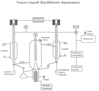
איור 1: תיאור המנגנון

מקדם פעילות מוגדר כיחס בין הפוגאציות של הרכיב בתערובת בפועל לפוגאציות של פתרון אידיאלי של אותו הרכב. Fugacity הוא נכס המשמש כדי להראות הבדלים בין פוטנציאלים כימיים במדינות סטנדרטיות. פאג’אציות שלב אדים יכולות לבוא לידי ביטוי במונחים של מקדם fugacity [φ: fiV = φi yi fi0V ], עם yi = שבר i בשלב האדים, ו- fi0V = fugacity מצב סטנדרטי אדים (fugacity של אדי רכיב טהור ב- T ו- P). עבור לחצים נמוכים, כמו בניסוי זה, φi = 1 ו- fi0V = P. fugacities שלב נוזלי יכול לבוא לידי ביטוי במונחים של מקדם פעילות γi: fiL = γi xi fi0L , עם xi = שבר i בשלב הנוזל, ו fi0L = fugacity מצב סטנדרטי נוזלי.

בלחץ הרוויה (Pis)של T זה, fugacity נוזלי הרכיב הטהור יהיה Pis,כי האדים והנוזל הטהורים נמצאים בשיווי משקל. מאז fugacities נוזלי הם רק פונקציות חלשות של לחץ, אנחנו יכולים להעריך את fugacity נוזלי הרכיב הטהור ב T ו- P (fi0L) כמו Pis,כל עוד ההבדל בין Pis ו- P אינו גדול. קירוב זה נקרא בדרך כלל “הזנחת תיקון פוינטינג”. אם הנסיינים משתמשים במנגנון VLE כדי למדוד את הרכבי האדים והנוזל הנמצאים בשיווי משקל, הנסיינים יכולים לחשב ישירות את מקדמי הפעילות המסופקים כדי למדוד גם P ו- T. T. יש למדוד כדי לקבוע PiS עבור כל i.

הלב של מכשיר VLE, המשמש בניסוי זה כדי לקבוע קומפוזיציות של תערובות, הוא משאבת Cottrell אשר “יורק” נוזל רותח לתוך תא מבודד היטב, שיווי משקל. שני שסתומי דגימה המופעלים מגנטית מאפשרים נסיגה של דגימות אדים נוזליות ומרוכזות. מאגר גדול מסייע לדכא פעימות לחץ במערכת כאשר שסתום הבקרה המתניע מתגמש, ומתנודות הנגרמות על ידי משאבת Cottrell. דליפה איטית יכולה לשמש ליצירת איזון בין קצב הנסיגה של האוויר לבין קצב הכניסה של האוויר כדי לשמור על לחץ מתמיד, במידת הצורך.

דרך דומה לפתור שיווי משקל נוזלי אדים היא להשתמש במגוון דגמים. החוק של ראול, החוק של דלטון, והחוק של הנרי הם כולם מודלים תיאורטיים שיכולים למצוא את נתוני ריכוז שיווי המשקל הנוזלי של האדים. כל שלושת המודלים קשורים מידתיות של לחצים חלקיים, לחץ מוחלט, ושברירי שומה של חומרים. המשוואה של וילסון הוכחה כמדויקת לנוזלים מטעים, בעוד שהיא לא מורכבת מדי. בנוסף, המודל של וילסון משלב מקדמי פעילות כדי להסביר סטייה מערכים אידיאליים.

Procedure

1. תראש המערכת לפרוק את מערכת VLE באמצעות שסתום 3-כיווני פורקן / בקרה רכוב על מסגרת המנגנון, ו (במידת הצורך) על ידי ניקוז נוזל מתוך המערכת לתוך בקבוקון פסולת. הסר את הצינורות לדוגמה ולהחליף עם צינורות נקיים (במידת הצורך). הנוזל לא יתנקז לחלוטין מהמערכת. עבור ההפעלה הראשונה של ניסויים, למלא מחדש דרך שסתום הכניסה עם תערובת של בערך (vol %) 50% מתנול, 30% איזופרופנול ו 20% מים. בשבוע השני, למלא עם בערך 25% מתנול, 45% איזופרופנול ו 30% מים. במשך השבוע השלישי, למלא עם כל נוזל שאתה צריך לחזור. הקיבולת הנוזלית הכוללת היא כ 130 ס”מ3. מלא בנוזל ממש מתחת לנקודה שבה משאבת Cottrell מצטלבת עם ז’קט ואקום. מעט מדי נוזל יגרום למערכת לדרוש שיעורי רתיחה גבוהים מאוד כדי לקבל מספיק נוזל כדי “לירוק” (כאשר נוזל קופץ תוך כדי רותחים בעוצמה). השתמש ויוצקים את הנוזל לתוך יציאת התוספת בחלק העליון של תא שיווי המשקל. סגור את הנמל. בדוק את הלחץ הברומטרי עם מנורת הכספת על הקיר. התאם את ה”אפס” במד הלחץ הדיגיטלי כך שיתאים (במידת הצורך). החלף את שסתום האוורור המשולש ל”שליטה”, והפעל את משאבת הוואקום ובקר הלחץ. פתח את שסתום המצערת על בקר הלחץ מספר סיבובים והתבונן בלחץ יורד במהירות. שים לב ללחץ על מד הלחץ הדיגיטלי. הגדר את נקודת לחץ הבקרה על בקר הלחץ כדי להשיג ~ 700 מ”מ Hg. להקשיב ללחיצה על שסתום הבקרה. ברגע שנקודת הבקרה תגיע, הרעש ממשאבת הוואקום יהיה שונה לחלוטין. בשלב זה, עם שסתום המצערת נפתח מספר סיבובים, בכל פעם שסתום הבקרה נפתח, יותר מדי אוויר נזרק למשאבת ואקום ואת הלחץ יורד מתחת 700 מ”מ לפני מתאושש לאט. סגור את שסתום המצערת לחלוטין, ולאחר מכן לפתוח אותו על 1/2 סיבוב. המתן עד שסתום הבקרה להתחיל ללחוץ שוב, ולאחר מכן לסגור את שסתום המצערת במרווחים קטנים עד הלחץ משתנה רק ~ 0.5 מ”מ כ”ג או פחות כאשר השסתום פתוח. בצע התאמות קלות לנקודת הבקרה או שסתום הדליפה לפי הצורך כדי לשמור על קרוב מאוד 700 מ”מ ל’ג. ברגע שהתערובת היא בתוך ±10 מ”מ כ”ג של 700 מ”מ כ”ג, להפעיל את כוח התנור, כוח המעטפת חימום, מים מעבים stirrer מגנטי. נסה 25-30% כוח תנור ו 1.5-2 הופך כוח המעטפת להתחיל. המנגנון ידרוש 20 דקות או פחות כדי להתקרב לשיווי משקל. תמשיך להתאים את הלחץ בתקופה זו. 2. הפעלת הניסוי עם הרתיחה, משאבת Cottrell תתחיל לירוק נוזל ונוזל ניתן לראות נוטף בחזרה לתוך תא הרותח. אדים מרוכזים ידרשו זמן רב יותר להופיע. כאשר שיווי משקל הוא הגיע, הנסיינים צריכים לראות טפטופים קבועים של אדים מרוכזים (2 – 3 טיפות / s) וחזר נוזל (2 – 3 טיפות / s). הטמפרטורה צריכה להיות יציבה כדי ± 0.03 מעלות צלזיוס והלחץ צריך להיות יציב ב 700.0 ± 0.5 מ”מ ל”ג. כאשר תנאים אלה נקבעו לפחות 2 דקות (בערך), שיווי משקל מושגת. פתח את השסתומים המגנטיים (מסומן “1” ו “2” על הבקר) 4 או 5 פעמים כל אחד במשך זמן מספיק כדי לאסוף כ 0.5 ס”מ3 של נוזל בכל צינור מדגם, ולסגור את הצינורות. אם שסתום אינו מגיב ללחצן שלו, נסה להפוך את מתג ההפעלה עבור הבקר כבוי ולאחר מכן מופעל. מדגם ראשון זה ישמש לשטוף את הצינורות ואת מערכת המשלוח יהיה מושלך. כביסה מחליפה את כל הכימיקל שנותר בצדי הצינורות באותו חומר כימי שנדגם, כך שזה לא ישפיע על הרכב הבדיקה. לרגע לכבות את הכוח לתנור, לחכות 30 s עבור רותחים להתפוגג, ולאחר מכן לפרוק את המערכת עם שסתום 3-כיווני פורקן / שליטה. הסר את צינורות מדגם, מערבולת כמה פעמים, ואז לזרוק אותם לתוך סיר הפסולת. להתאים מחדש את צינורות המדגם במערכת, להפוך את שסתום האוורור בחזרה “שליטה”, להפעיל את הכוח בחזרה לתנור, ולחכות שיווי המשקל כדי להפוך מחדש. זה ייקח רק כמה דקות אם המנגנון לא מתקרר. הבדל קל בטמפרטורה ניתן לראות כאשר שיווי המשקל הוא מחדש. זה יכול להיות בגלל הפרעה קלה של הרכב הכולל עקב דגימה. לאחר שיווי המשקל הוא מחדש, לקחת שתי דגימות חדשות. יש שני בקבוקונים מסומנים עם ספטה חדשה מוכנה. לאחר נטילת ~ 0.5 ס”מ3 דגימות בכל צינור שוב, לכבות את התנור, לפרוק את המערכת, להסיר את צינורות מדגם ולשפוך אותם לתוך הבקבוקונים. לכסות את הבקבוקונים ולהחליף את הצינורות מדגם עם צינורות נקיים במידת הצורך. בעת ניתוח הדגימות, הכינו דגימה חדשה. מסננים כ-15 ס”מ3 נוזלים לכוב או לבקבוקון. הוסף ~ 20 ס”מ3 של מתנול טהור או 50/50 מתנול / איזופרופנול דרך יציאת המדגם. זה ייתן הרכב כולל חדש. ודא צינורות מדגם ריקים לחלוטין, ולאחר מכן לסגור את המערכת, לכבות את שסתום האוורור כדי “לשלוט”, ולהדליק את התנור בחזרה. אם יעבוד במהירות, שיווי המשקל יוקם מחדש במהירות. שים לב כי צריך להיות הבדל טמפרטורה מן המדגם הקודם. חזור על הליך שיווי משקל ודגימה כמו קודם, לזכור לקחת מדגם אחד לשטוף, ולאחר מכן לקחת את המדגם הסופי. המשך בניסויים על-ידי הוספת רכיבים. 12 נקודות נתונים מספיקות כדי לקבוע את מקדמי הפעילות ואת (בערך) מקדמי האינטראקציה הבינארית. 3. כיבוי המערכת כבה את התנורים. כאשר המנגנון מתחיל להתקרר, לכבות את stirrer ואת מי ה עיבוי. להחזיר את המערכת ללחץ אטמוספרי; להגדיר את הבקר >1020 mbar, לסגור את שסתום המצערת, להגדיר את שסתום משולש לפרוק ולפתוח את השסתום על הטנק. ברגע שהושג לחץ אטמוספרי, כבה את המשאבה. מסננים את הנוזל מהמאגר עד שהוא מגיע לרמת השסתום, אך משאירים את שאר הנוזל במאגר. סגור את שסתום 3 כיווני. 4. ניתוח באמצעות רגרסיה לא ליניארית וסכום סטנדרטי של פונקציית המטרה של שיורית בריבוע, השתמש במקדם הפעילות המחושב מהנתונים הגולמיים כדי לסגת מ- 6 הקבועים עבור משוואת וילסון הטרנרית (להלן), עבור מערכת זו. להעריך את איכות ההתאמה על ידי שיטות גרפיות וחישוב הסטיות היחסיות באחוז הממוצע (APRD), שהן שגיאות התאמה ממוצעות x 100. התכנסו לערכים האופטימליים האמיתיים מכמה כיוונים שונים במרחב פרמטרי התגובה באמצעות שיטה פקטורלית לניחושים הראשוניים. לחשב את הדיוק של מדידות GC על ידי שכפול מספיק מדגם GC אחד כדי לקבוע דיוק יחסי על פי t-statistic, ולהשתמש בדיוק כדי לקבוע אם לקבל / לדחות מדידת GC מסוימת על ידי בדיקת השערה מתאימה. השווה את הדיוק היחסי של מדידת GC ל- APRDs, ודון. דיווחו גם על הדיוק המוחלט של מדי הלחץ והטמפרטורה – קבעו אותם פעם ביום.

Results

The activity coefficients of the data do not show significant deviations from a mean value for each component (Table 1). This is as expected because for intermediate component compositions there are not large variations. However, components near 1 have γ's near 1. Low composition components have high γ's. Components highest in concentration in a mixture which will have a reduced deviation, therefore it will be closer to ideal (γ = 1). Components with lower concentrations in a mixture will have higher deviations, so their γ's will be greater than 1.

Table 1

Table 1: Results of each sampling of the experimental data.

The data were fit to Wilson model parameters and the coefficients were calculated (Table 2). A simple reduction in the sum of squared residuals between experimental and Wilson equation (1) activity coefficients was used. This was achieved using Excel's solver function. The parity plot shown relates the Wilson's Equation model activity coefficients to the experimentally found activity coefficients. The experimental activity coefficients were calculated and graphically compared to the calculated model coefficients.

Table 2

Table 2: Results of fitting the data to the Wilson model parameters.
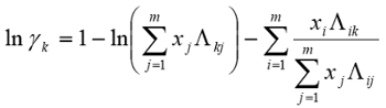
Equation 1 (1)

The parameter values found were the best fit (Table 3). Ideally the correlation is along the y=x line; however, a significant correlation resembling the ideal scenario was found (Figure 2). The activity coefficients of the data did not show significant deviations from a mean value for each component, as expected. A reduction in the sum of squared residuals between experimental and Wilson equation activity coefficients was used with Excel's solver function. The parity plot relates the Wilson's Equation model activity coefficients to the experimentally found activity coefficients.

Table 3

Table 3: Model parameters with water (a), MeOH (b), and IPA (c). The experimental values are compared to expected values.

Figure 2
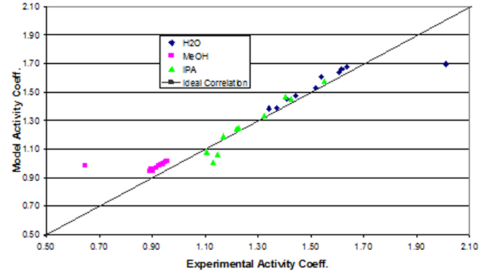
Figure 2: Depiction of the correlation between the experimental activity coefficients and the model activity coefficients.

Applications and Summary

This experiment demonstrated the equilibration of methanol – isopropanol – water vapor-liquid mixtures at a constant P = 700 mm Hg and how to measure temperature and composition and calculate activity coefficients. The activity coefficients of the data did not significantly deviate from a mean value for each component, as expected. A reduction in the sum of squared residuals between experimental and Wilson equation activity coefficients was used with Excel's solver function. The parity plot relates the Wilson's Equation model activity coefficients to the experimentally found activity coefficients.

In the petroleum industry, distillation is the primary process for separation of petroleum products. Many oil refineries use distillation for crude oil1. Light hydrocarbons are separated from heavier particles, separating based on boiling points1. Heavy materials like gas oils collect in the lower plates, while light materials like propane and butane rise up1. Hydrocarbons, such as gasoline, jet, and diesel fuels, are separated1. This process is often repeated many times to fully separate and refine the products1. Refineries run these processes at steady state, constantly creating new products at maximum capacity, so efficiency is key1. Chemical engineers working on these processes focus on optimizing the efficiency of the production1.

Tray distillation columns are also used to separate a variety of chemical products. Ethanol is one such product. Through closely related processes, a variety of products such as fuel-grade ethanol, beer, and liquor can all be distilled2. Specific amounts of alcohol can be separated from water in order to create a specific proof2. This process is limited to reducing the percentage of water in the product, but cannot completely eliminate it2. In order to remove water completely, azeotropic distillation is required, which uses extractor chemicals to separate water from ethanol2.

References

  1. About the Refinery." Processing & Refining Crude Oil. Chevron.com, n.d. Web. 17 Nov. 2016.
  2. Madson, PW. Ethanol Distillation: The Fundamentals. Cincinnati: Katzen International, n.d. Print. Accessed from Web. 01 Oct. 2016.

Transcript

Understanding the distribution of chemical components in both the vapor and liquid phase, called vapor-liquid equilibrium is essential to the design, operation, and analysis of many engineering processes. Vapor-liquid equilibrium or VLE is a state at which a pure component or mixture exists in both the liquid and vapor phases. The phases are at equilibrium meaning that there were no changes in the macroscopic properties of the system over time. Single component VLE is simple to visualize. Take for example water which is at equilibrium in the vapor and liquid phase at 100 degrees Celsius and one atm. Above this temperature water is a vapor. Below it, water is a liquid. However, engineers generally encounter processes with mixtures in equilibrium making the analysis of VLE more complex and therefore essential to process design. This video will illustrate the principles behind vapor-liquid equilibrium of mixtures and demonstrate how to analyze the VLE of a mixture in the laboratory. Finally, some applications of VLE in the chemical engineering field will be introduced.

When a heated mixture is in a vapor-liquid equilibrium, the vapor and liquid phases generally do not have the same composition. The substance with the lower boiling point will have a higher concentration in the vapor than the substance with the higher boiling point. Thus, engineers refer to components in each phase by their mole fraction where xi is the mole fraction of species i in the liquid and yi is the mole fraction of species i in the vapor phase. This relationship is often depicted using an xy curve like the one shown here for a mixture of two components which illustrates the relationship between each component in each phase. A starting point for all VLE calculations is the simple equilibrium criterion where the fugacity of the species in the vapor equals the fugacity of the species in the liquid. Fugacity is a property related to the exponential difference between the real and ideal gas Gibbs energies. The vapor phase fugacity is equal to the mole fraction of species i in the vapor phase times the pure component vapor fugacity. The expression can be simplified as the pure component vapor fugacity is approximately equal to pressure at low pressure. Liquid phase fugacities are expressed in terms of an activity coefficient, gamma. The activity coefficient is defined as the ratio of a component’s fugacity in an actual mixture to the fugacity of an ideal solution of the same composition. At the saturation vapor pressure the pure component liquid fugacity would equal the saturation vapor pressure because the pure vapor and liquid are in equilibrium there. Finally, since the liquid and vapor fugacities are equal, we can further simplify the relationship as shown which is also known as Raoult’s law. The saturation vapor pressure is often calculated using the Antoine equation where the constants A, B, and C are species-specific and can be found in the literature. Thus, if we measure the compositions of the vapor and liquid which are in equilibrium, we can directly calculate the activity coefficients by measuring temperature and pressure and therefore the saturation vapor pressure. In this experiment a ternary mixture of methanol, isopropyl alcohol and water will be investigated. Various compositions of the mixture are boiled in a VLE apparatus and the lower boiling point components vaporize and are collected in a separate container while the liquid gathers back into the initial sample vessel. Once equilibrium is reached, the liquid and condensed vapor fractions are collected and analyzed with gas chromatography. Using temperature and the liquid and vapor mole fractions the activity coefficients can be calculated. Now that you’ve been introduced to the concepts of VLE and the testing apparatus, let’s see how to carry out the experiment in the laboratory.

To start, drain any liquid out of the system into a waste flask. Keep in mind that the liquid may not completely drain. For the first run add a mixture of 50% methanol, 30% IPA and 20% water through the opening at the top. After filling the mixture, turn on the heater power and condenser water. The apparatus will require roughly 20 minutes to approach equilibrium. The system is now ready to begin the experiment.

When the sample begins boiling, release the stopper to vent the inert outlet of the system. Condensed vapor will start collecting. When equilibrium is reached, steady drips of condensed vapor and returns liquid should be observed. With the temperature stable to within 0.3 degrees for 10 minutes, collect about 1/2 milliliter of liquid in sample vials from both the condensed vapor and the boiling liquid. Drain the condensed vapor from the last sample. Then add a new sample consisting of either 20 milliliters of pure methanol or 50-50 methanol-isopropanol through the sample port. This will give a new overall composition. Reestablish the equilibrium as performed before, however expect a temperature difference from the previous sample. Repeat the equilibration and sampling procedure as before, and then collect the sample to be analyzed. Continue the experiment using different mixtures of the three components. 12 points are sufficient to determine the activity coefficients and the binary interaction coefficients. When all the mixtures have been run, shut down the system by turning off the heaters. When the apparatus begins to cool, shut off the condenser water. Finally measure the composition of each liquid and vapor sample with the gas chromatograph or GC.

Using the system temperature and the liquid and vapor mole fractions acquired from GC, calculate the activity coefficients. This first requires that the saturation pressure is calculated using the Antoine equation where the constants A, B and C for each component can be found in the literature. Now we can use the calculated activity coefficients to correlate the data to a model. We will use the Wilson equation for a ternary mixture which accounts for deviations from ideality in a mixture. The nine lambda constants are the Wilson constants which equal one when i equals j. For each ij pair, there are two different constants. Use a nonlinear regression and a standard sum of squares residual function to determine the six remaining Wilson constants using the mole fraction data from the experiment. The Wilson constants are then used to determine the expected activity coefficients for each component of each sample. Here we show the modeled activity coefficient plotted against the experimental activity coefficients. Ideally, the modeled and experimental activity coefficients would fall along the y equals x line. As you can see in general, the modeled and experimental values fit along this line showing that the model is a good fit to the real system.

Understanding and manipulating the vapor-liquid equilibrium of mixtures is a vital component to a range of processes especially separations. Distillation columns separate mixtures based on their volatility with different compositions of each component in the liquid and vapor phrases on each tray. The more volatile component is vaporized and collected at the top of the column, while the less volatile component remains liquid and is collected at the bottom. VLE data of the components of the mixture is used to determine the number of trays needed to achieve separation in a distillation column. This helps engineers optimize the separation process while keeping operating costs low. Another valuable separation technique using VLE is flash separation. Flash separation is based on the fact that a liquid at a pressure equal to or greater than its bubble point pressure flashes meaning that it partially evaporates when the pressure is reduced. The feed is preheated thus consisting of some liquid and some vapor in equilibrium. It then flows through a pressure reducing valve into the separator. The degree of vaporization and therefore the amount of the solute in the vapor or liquid phases depends on the initial state of the feed stream.

You’ve just watched Jove’s introduction to vapor-liquid equilibrium. You should now understand the concepts behind VLE, how it’s measured in the laboratory, and some of its uses in engineering processes. Thanks for watching.

Tags

Cite This
JoVE Science Education Database. JoVE Science Education. Vapor-liquid Equilibrium. JoVE, Cambridge, MA, (2023).