JoVE Science Education
Chemical Engineering
This content is Free Access.
JoVE Science Education Chemical Engineering
Vapor-liquid Equilibrium
  • 00:07Overview
  • 01:36Principles of Vapor-liquid Equilibrium
  • 05:15Priming the VLE System
  • 06:00Running VLE Experiments
  • 07:52Results
  • 09:33Applications
  • 11:09Summary

Equilíbrio vapor-líquido

English

Share

Overview

Fonte: Michael G. Benton e Kerry M. Dooley, Departamento de Engenharia Química, Louisiana State University, Baton Rouge, LA

O equilíbrio vapor-líquido é primordial em aplicações de engenharia, como destilação, modelagem ambiental e design geral de processos. Entender as interações dos componentes em uma mistura é muito importante na concepção, operação e análise desses separadores. O coeficiente de atividade é uma excelente ferramenta para relacionar interações moleculares à composição da mistura. Encontrar os parâmetros de interação molecular permite a previsão futura dos coeficientes de atividade para uma mistura usando um modelo.

O equilíbrio vapor-líquido é um fator crítico em processos comuns na indústria química, como a destilação. Destilação é o processo de separação de líquidos pelo ponto de ebulição. Uma mistura líquida é alimentada em uma unidade de destilação ou coluna, em seguida, fervida. Os dados de equilíbrio vapor-líquido são úteis para determinar como as misturas líquidas se separarão. Como os líquidos têm diferentes pontos de ebulição, um líquido ferverá em um vapor e subirá na coluna, enquanto o outro permanecerá como líquido e drene pela unidade. O processo é muito importante em uma variedade de indústrias.

Neste experimento, os coeficientes de atividade de misturas de várias composições de metanol, isopropanol e água deionizada serão obtidos utilizando um aparelho de equilíbrio vapor-líquido e cromatógrafo gasoso. Além disso, os parâmetros de interação binária do sistema serão determinados usando a equação de Wilson e os coeficientes de atividade.

Principles

O equilíbrio vapor-líquido é um estado no qual existe um componente ou mistura pura em fases líquidas e de vapor, com equilíbrio mecânico e térmico e sem transferência de massa líquida entre as duas fases. Vapor e líquido são separados pela gravidade e calor (Figura 1). A mistura líquida é inserida no sistema, que é colocado em um estado de vácuo com uma bomba de vácuo. O vapor é condensado e devolvido para misturar com o líquido, que é então passado de volta para a câmara fervente. Diferenças no ponto de ebulição resultam em alguma separação da mistura. O ponto de ebulição da água é maior do que o dos componentes adicionados, de modo que os componentes voláteis começam a evaporar.

Figure 1
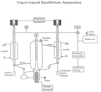
Figura 1: Uma representação do aparelho

Um coeficiente de atividade é definido como a razão da fugacidade de um componente em uma mistura real à fugacidade de uma solução ideal da mesma composição. Fugacity é uma propriedade usada para mostrar diferenças entre potenciais químicos em estados padrão. As fugacidades da fase de vapor podem ser expressas em termos de coeficiente fugacidade [φ: fiV = φi yi fi0V ], com yi = fração mol de i na fase de vapor, e fi0V = o estado de vapor fugacity (a fugacidade do vapor de componente puro em T e P). Para baixas pressões, como neste experimento, φi = 1 e fi0V = P. As fugacidades de fase líquida podem ser expressas em termos de coeficiente de atividade γi: fiL = γi xi fi0L , com xi = fração mol de i na fase líquida, e fi0L = o estado líquido fugacity.

Na pressão de saturação (Pis)deste T, o componente puro fugacity líquido seria Pis,porque o vapor puro e o líquido estão em equilíbrio. Como as fugacidades líquidas são apenas funções fracas de pressão, podemos aproximar o componente puro líquido fugacity em T e P (fi0L) como Pis,desde que a diferença entre Pis e P não seja grande. Essa aproximação é geralmente chamada de “negligenciar a correção poynting”. Se os experimentadores usarem um aparelho VLE para medir as composições do vapor e do líquido que estão em equilíbrio, os experimentadores podem calcular diretamente os coeficientes de atividade fornecidos para medir também P e T. T devem ser medidos para determinar PiS para todos i.

O coração do dispositivo VLE, usado neste experimento para determinar composições de misturas, é uma bomba Cottrell que “cospe” líquido fervente em uma câmara de equilíbrio bem isolada. Duas válvulas de amostragem operadas magneticamente permitem a retirada de amostras de vapor líquido e condensado. Um grande reservatório ajuda a amortecer os pulsos de pressão no sistema à medida que a válvula de controle desligada muda, e a partir de flutuações causadas pela bomba de Cottrell. Um vazamento lento pode ser usado para criar um equilíbrio entre a taxa de retirada de ar e a taxa de entrada de ar para manter uma pressão constante, se necessário.

Uma maneira comparável de resolver para o equilíbrio vapor-líquido é usar uma variedade de modelos. A lei de Raoult, a lei de Dalton e a lei de Henry são todos modelos teóricos que podem encontrar os dados de concentração de equilíbrio vapor-líquido. Todos os três modelos estão relacionados com a proporcionalidade de pressões parciais, pressão total e frações de substâncias. A equação de Wilson tem sido provada como precisa para líquidos miscíveis, embora não seja excessivamente complexa. Além disso, o modelo de Wilson incorpora coeficientes de atividade para contabilizar o desvio dos valores ideais.

Procedure

1. Priming o sistema Desabafe o sistema VLE usando a válvula de ventilação/controle de 3 vias montada na estrutura do aparelho e (se necessário) drenando líquido do sistema em um frasco de resíduos. Remova os tubos de amostra e substitua por tubos limpos (se necessário). O líquido não vai drenar completamente para fora do sistema. Para a primeira execução de experimentos, refile através da válvula de entrada com uma mistura de aproximadamente (vol %) 50% de metanol, 30% isopropanol e 20% de água. Pela segunda semana, refil com cerca de 25% de metanol, 45% isopropanol e 30% de água. Para a terceira semana, refile com o líquido que você precisa repetir. A capacidade líquida total é de aproximadamente 130 cm3. Encha com líquido logo abaixo do local onde a bomba de Cottrell se cruza com a jaqueta de vácuo. Muito pouco líquido fará com que o sistema exija taxas de ebulição muito altas para obter líquido suficiente para “cuspir” (quando o líquido estoura enquanto ferve intensamente). Use um béquer e despeje o líquido na porta de adição na parte superior da câmara de equilíbrio. Feche o porto. Verifique a pressão barométrica com o manômetro de mercúrio na parede. Ajuste o “zero” no medidor de pressão digital para combinar (se necessário). Mude a válvula de ventilação de três vias para “controle” e inicie a bomba de vácuo e o controlador de pressão. Abra a válvula do acelerador no controlador de pressão várias voltas e observe a pressão cair rapidamente. Observe a pressão no medidor de pressão digital. Ajuste o ponto de ajuste de pressão de controle no controlador de pressão para obter ~ 700 mm Hg. Ouça para clicar na válvula de controle. Uma vez alcançado o ponto de controle, o ruído da bomba de vácuo será audivelmente diferente. Neste ponto, com a válvula do acelerador aberta várias voltas, toda vez que a válvula de controle se abre, muito ar é despejado na bomba de vácuo e a pressão cai abaixo de 700 mm antes de se recuperar lentamente. Feche completamente a válvula do acelerador e abra-a por volta de 1/2. Aguarde que a válvula de controle comece a clicar novamente, em seguida, feche a válvula do acelerador em pequenos incrementos até que a pressão flutua apenas ~0,5 mmHg ou menos quando a válvula estiver aberta. Faça pequenos ajustes no ponto de controle ou na válvula de escape, conforme necessário, para manter muito perto de 700 mmHg. Uma vez que a mistura esteja dentro de ±10 mmHg de 700 mmHg, ligue a potência do aquecedor, aquecendo a potência do manto, a água do condensador e o agitador magnético. Tente 25-30 % de potência do aquecedor e 1,5-2 vira potência de manto para iniciar. O aparelho exigirá 20 minutos ou menos para se aproximar do equilíbrio. Continue ajustando a pressão durante este tempo. 2. Executando o experimento Após ferver, a bomba de Cottrell começará a cuspir líquido e o líquido pode ser visto pingando de volta para a câmara de ebulição. Vapor condensado exigirá mais tempo para aparecer. Quando o equilíbrio é atingido, os experimentadores devem ver gotejamentos constantes de vapor condensado (2 – 3 gotas/s) e líquido devolvido (2 – 3 gotas/s). A temperatura deve ser estável a ± 0,03 ºC e a pressão deve ser estável a 700,0 ± 0,5 mmHg. Quando essas condições foram estabelecidas por pelo menos 2 minutos (ou mais), o equilíbrio é alcançado. Abra as válvulas magnéticas (marcadas “1” e “2” no controlador) 4 ou 5 vezes cada uma por tempo suficiente para coletar cerca de0,5 cm de líquido em cada tubo de amostra, e fechar os tubos. Se uma válvula não responder ao botão, tente ligar o interruptor de alimentação para o controlador. Esta primeira amostra será usada para lavar os tubos e o sistema de entrega e será descartada. A lavagem substitui qualquer produto químico restante nas laterais dos tubos pelo mesmo produto químico que está sendo amostrado, de modo que não afetará a composição do teste. Desligue momentaneamente a energia do aquecedor, espere 30 s para que a ebulição diminua e, em seguida, desligue o sistema com a válvula de ventilação/controle de 3 vias. Remova os tubos de amostra, gire algumas vezes e despeje-os no pote de lixo. Recoloque os tubos de amostra no sistema, gire a válvula de ventilação para trás para “controle”, ligue a energia de volta ao aquecedor e aguarde que o equilíbrio seja restabelecido. Isso só vai demorar alguns minutos se o aparelho não esfriar. Uma pequena diferença de temperatura pode ser observada quando o equilíbrio é restabelecido. Isso pode ser devido a uma leve perturbação da composição geral devido à amostragem. Uma vez que o equilíbrio seja restabelecido, pegue duas novas amostras. Tenha dois frascos rotulados com novo septa pronto. Depois de colher ~0,5 cm3 amostras em cada tubo novamente, desligue o aquecedor, desligue o sistema, remova os tubos de amostra e despeje-os nos frascos. Tampe os frascos e substitua os tubos de amostra por tubos limpos, se necessário. Ao analisar as amostras, prepare uma nova amostra. Escorra ~15 cm3 de líquido em um béquer ou frasco. Adicione ~20 cm3 de metanol puro ou 50/50 metanol/isopropanol através da porta de amostra. Isso dará uma nova composição geral. Certifique-se de que os tubos de amostra estão completamente vazios, em seguida, feche o sistema, desligue a válvula de ventilação para “controlar” e ligue o aquecedor novamente. Se funcionar rapidamente, o equilíbrio será restabelecido rapidamente. Note que deve haver uma diferença de temperatura em da amostra anterior. Repita o procedimento de equilíbrio e amostragem como antes, lembrando de colher uma amostra para lavar e, em seguida, pegue a amostra final. Continue os experimentos adicionando componentes(s). Doze pontos de dados são suficientes para determinar os coeficientes de atividade e (aproximadamente) os coeficientes de interação binária. 3. Desligar o sistema Desligue os aquecedores. Quando o aparelho começar a esfriar, desligue o agitador e a água do condensador. Devolver o sistema à pressão atmosférica; ajuste o controlador >1020 mbar, feche a válvula do acelerador, ajuste a válvula de três vias para ventilar e abra a válvula no tanque. Uma vez que a pressão atmosférica tenha sido atingida, desligue a bomba. Escorra o líquido do reservatório até atingir o nível da válvula, mas deixe o resto do líquido no reservatório. Feche a válvula de 3 vias. 4. Análise Utilizando regressão não linear e uma soma padrão de função objetiva de resíduos quadrados, utilize os coeficientes de atividade computados a partir dos dados brutos para regredir as 6 constantes para a equação ternary wilson (abaixo), para este sistema. Avalie a qualidade do ajuste por métodos gráficos e compute os desvios relativos por cento médios (APRD), que são erros de ajuste médios x 100. Convergir sobre os verdadeiros valores ideais de várias direções diferentes no espaço do parâmetro de resposta usando um método fatorial para os palpites iniciais. Calcule a precisão das medições de GC replicando suficientemente uma amostra de GC para determinar as precisão relativas de acordo com a t-estatística, e use as precisão para determinar se aceita ou rejeita uma determinada medição de GC por teste de hipótese apropriado. Compare as precisão relativas da medição gc com os APRDs e discuta. Também informe as precisão absolutas dos medidores de pressão e temperatura – determine estas uma vez por dia.

Results

The activity coefficients of the data do not show significant deviations from a mean value for each component (Table 1). This is as expected because for intermediate component compositions there are not large variations. However, components near 1 have γ's near 1. Low composition components have high γ's. Components highest in concentration in a mixture which will have a reduced deviation, therefore it will be closer to ideal (γ = 1). Components with lower concentrations in a mixture will have higher deviations, so their γ's will be greater than 1.

Table 1

Table 1: Results of each sampling of the experimental data.

The data were fit to Wilson model parameters and the coefficients were calculated (Table 2). A simple reduction in the sum of squared residuals between experimental and Wilson equation (1) activity coefficients was used. This was achieved using Excel's solver function. The parity plot shown relates the Wilson's Equation model activity coefficients to the experimentally found activity coefficients. The experimental activity coefficients were calculated and graphically compared to the calculated model coefficients.

Table 2

Table 2: Results of fitting the data to the Wilson model parameters.
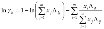
Equation 1 (1)

The parameter values found were the best fit (Table 3). Ideally the correlation is along the y=x line; however, a significant correlation resembling the ideal scenario was found (Figure 2). The activity coefficients of the data did not show significant deviations from a mean value for each component, as expected. A reduction in the sum of squared residuals between experimental and Wilson equation activity coefficients was used with Excel's solver function. The parity plot relates the Wilson's Equation model activity coefficients to the experimentally found activity coefficients.

Table 3

Table 3: Model parameters with water (a), MeOH (b), and IPA (c). The experimental values are compared to expected values.

Figure 2
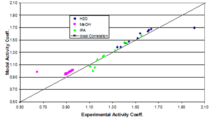
Figure 2: Depiction of the correlation between the experimental activity coefficients and the model activity coefficients.

Applications and Summary

This experiment demonstrated the equilibration of methanol – isopropanol – water vapor-liquid mixtures at a constant P = 700 mm Hg and how to measure temperature and composition and calculate activity coefficients. The activity coefficients of the data did not significantly deviate from a mean value for each component, as expected. A reduction in the sum of squared residuals between experimental and Wilson equation activity coefficients was used with Excel's solver function. The parity plot relates the Wilson's Equation model activity coefficients to the experimentally found activity coefficients.

In the petroleum industry, distillation is the primary process for separation of petroleum products. Many oil refineries use distillation for crude oil1. Light hydrocarbons are separated from heavier particles, separating based on boiling points1. Heavy materials like gas oils collect in the lower plates, while light materials like propane and butane rise up1. Hydrocarbons, such as gasoline, jet, and diesel fuels, are separated1. This process is often repeated many times to fully separate and refine the products1. Refineries run these processes at steady state, constantly creating new products at maximum capacity, so efficiency is key1. Chemical engineers working on these processes focus on optimizing the efficiency of the production1.

Tray distillation columns are also used to separate a variety of chemical products. Ethanol is one such product. Through closely related processes, a variety of products such as fuel-grade ethanol, beer, and liquor can all be distilled2. Specific amounts of alcohol can be separated from water in order to create a specific proof2. This process is limited to reducing the percentage of water in the product, but cannot completely eliminate it2. In order to remove water completely, azeotropic distillation is required, which uses extractor chemicals to separate water from ethanol2.

References

  1. About the Refinery." Processing & Refining Crude Oil. Chevron.com, n.d. Web. 17 Nov. 2016.
  2. Madson, PW. Ethanol Distillation: The Fundamentals. Cincinnati: Katzen International, n.d. Print. Accessed from Web. 01 Oct. 2016.

Transcript

Understanding the distribution of chemical components in both the vapor and liquid phase, called vapor-liquid equilibrium is essential to the design, operation, and analysis of many engineering processes. Vapor-liquid equilibrium or VLE is a state at which a pure component or mixture exists in both the liquid and vapor phases. The phases are at equilibrium meaning that there were no changes in the macroscopic properties of the system over time. Single component VLE is simple to visualize. Take for example water which is at equilibrium in the vapor and liquid phase at 100 degrees Celsius and one atm. Above this temperature water is a vapor. Below it, water is a liquid. However, engineers generally encounter processes with mixtures in equilibrium making the analysis of VLE more complex and therefore essential to process design. This video will illustrate the principles behind vapor-liquid equilibrium of mixtures and demonstrate how to analyze the VLE of a mixture in the laboratory. Finally, some applications of VLE in the chemical engineering field will be introduced.

When a heated mixture is in a vapor-liquid equilibrium, the vapor and liquid phases generally do not have the same composition. The substance with the lower boiling point will have a higher concentration in the vapor than the substance with the higher boiling point. Thus, engineers refer to components in each phase by their mole fraction where xi is the mole fraction of species i in the liquid and yi is the mole fraction of species i in the vapor phase. This relationship is often depicted using an xy curve like the one shown here for a mixture of two components which illustrates the relationship between each component in each phase. A starting point for all VLE calculations is the simple equilibrium criterion where the fugacity of the species in the vapor equals the fugacity of the species in the liquid. Fugacity is a property related to the exponential difference between the real and ideal gas Gibbs energies. The vapor phase fugacity is equal to the mole fraction of species i in the vapor phase times the pure component vapor fugacity. The expression can be simplified as the pure component vapor fugacity is approximately equal to pressure at low pressure. Liquid phase fugacities are expressed in terms of an activity coefficient, gamma. The activity coefficient is defined as the ratio of a component’s fugacity in an actual mixture to the fugacity of an ideal solution of the same composition. At the saturation vapor pressure the pure component liquid fugacity would equal the saturation vapor pressure because the pure vapor and liquid are in equilibrium there. Finally, since the liquid and vapor fugacities are equal, we can further simplify the relationship as shown which is also known as Raoult’s law. The saturation vapor pressure is often calculated using the Antoine equation where the constants A, B, and C are species-specific and can be found in the literature. Thus, if we measure the compositions of the vapor and liquid which are in equilibrium, we can directly calculate the activity coefficients by measuring temperature and pressure and therefore the saturation vapor pressure. In this experiment a ternary mixture of methanol, isopropyl alcohol and water will be investigated. Various compositions of the mixture are boiled in a VLE apparatus and the lower boiling point components vaporize and are collected in a separate container while the liquid gathers back into the initial sample vessel. Once equilibrium is reached, the liquid and condensed vapor fractions are collected and analyzed with gas chromatography. Using temperature and the liquid and vapor mole fractions the activity coefficients can be calculated. Now that you’ve been introduced to the concepts of VLE and the testing apparatus, let’s see how to carry out the experiment in the laboratory.

To start, drain any liquid out of the system into a waste flask. Keep in mind that the liquid may not completely drain. For the first run add a mixture of 50% methanol, 30% IPA and 20% water through the opening at the top. After filling the mixture, turn on the heater power and condenser water. The apparatus will require roughly 20 minutes to approach equilibrium. The system is now ready to begin the experiment.

When the sample begins boiling, release the stopper to vent the inert outlet of the system. Condensed vapor will start collecting. When equilibrium is reached, steady drips of condensed vapor and returns liquid should be observed. With the temperature stable to within 0.3 degrees for 10 minutes, collect about 1/2 milliliter of liquid in sample vials from both the condensed vapor and the boiling liquid. Drain the condensed vapor from the last sample. Then add a new sample consisting of either 20 milliliters of pure methanol or 50-50 methanol-isopropanol through the sample port. This will give a new overall composition. Reestablish the equilibrium as performed before, however expect a temperature difference from the previous sample. Repeat the equilibration and sampling procedure as before, and then collect the sample to be analyzed. Continue the experiment using different mixtures of the three components. 12 points are sufficient to determine the activity coefficients and the binary interaction coefficients. When all the mixtures have been run, shut down the system by turning off the heaters. When the apparatus begins to cool, shut off the condenser water. Finally measure the composition of each liquid and vapor sample with the gas chromatograph or GC.

Using the system temperature and the liquid and vapor mole fractions acquired from GC, calculate the activity coefficients. This first requires that the saturation pressure is calculated using the Antoine equation where the constants A, B and C for each component can be found in the literature. Now we can use the calculated activity coefficients to correlate the data to a model. We will use the Wilson equation for a ternary mixture which accounts for deviations from ideality in a mixture. The nine lambda constants are the Wilson constants which equal one when i equals j. For each ij pair, there are two different constants. Use a nonlinear regression and a standard sum of squares residual function to determine the six remaining Wilson constants using the mole fraction data from the experiment. The Wilson constants are then used to determine the expected activity coefficients for each component of each sample. Here we show the modeled activity coefficient plotted against the experimental activity coefficients. Ideally, the modeled and experimental activity coefficients would fall along the y equals x line. As you can see in general, the modeled and experimental values fit along this line showing that the model is a good fit to the real system.

Understanding and manipulating the vapor-liquid equilibrium of mixtures is a vital component to a range of processes especially separations. Distillation columns separate mixtures based on their volatility with different compositions of each component in the liquid and vapor phrases on each tray. The more volatile component is vaporized and collected at the top of the column, while the less volatile component remains liquid and is collected at the bottom. VLE data of the components of the mixture is used to determine the number of trays needed to achieve separation in a distillation column. This helps engineers optimize the separation process while keeping operating costs low. Another valuable separation technique using VLE is flash separation. Flash separation is based on the fact that a liquid at a pressure equal to or greater than its bubble point pressure flashes meaning that it partially evaporates when the pressure is reduced. The feed is preheated thus consisting of some liquid and some vapor in equilibrium. It then flows through a pressure reducing valve into the separator. The degree of vaporization and therefore the amount of the solute in the vapor or liquid phases depends on the initial state of the feed stream.

You’ve just watched Jove’s introduction to vapor-liquid equilibrium. You should now understand the concepts behind VLE, how it’s measured in the laboratory, and some of its uses in engineering processes. Thanks for watching.

Tags

Cite This
JoVE Science Education Database. JoVE Science Education. Vapor-liquid Equilibrium. JoVE, Cambridge, MA, (2023).