JoVE Science Education
Microbiology
A subscription to JoVE is required to view this content.  Sign in or start your free trial.
JoVE Science Education Microbiology
Growth Curves: Generating Growth Curves Using Colony Forming Units and Optical Density Measurements
  • 00:01Concepts
  • 03:44Set-Up
  • 08:52Data Analysis and Results

עקומות צמיחה: יצירת עקומות צמיחה באמצעות יחידות יוצרות מושבה ומדידות צפיפות אופטית

English

Share

Overview

מקור: אנדרו ג’יי ואן אלסט1, ריאנון מ. לה-ווק1, נטליה מרטין1, וויקטור ג’יי דיריטה1
1 המחלקה למיקרוביולוגיה וגנטיקה מולקולרית, אוניברסיטת מדינת מישיגן, מזרח לנסינג, מישיגן, ארצות הברית

עקומות גדילה מספקות מידע רב ערך על קינטיקה של גדילה חיידקית ופיזיולוגיה של תאים. הם מאפשרים לנו לקבוע כיצד חיידקים מגיבים בתנאי גדילה משתנים, כמו גם להגדיר פרמטרי צמיחה אופטימליים עבור חיידק נתון. עקומת צמיחה ארכיטיפית מתקדמת דרך ארבעה שלבים של צמיחה: פיגור, מעריכי, נייח ומוות (1).

Figure 1
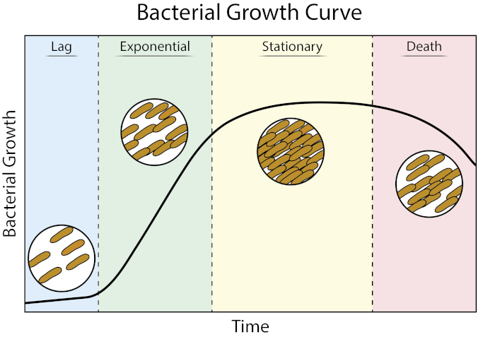
איור 1: עקומת גדילה חיידקית. חיידקים הגדלים בתרבות האצווה מתקדמים בארבעה שלבים של צמיחה: עיכוב, מעריכי, נייח ומוות. שלב ההשהיה הוא פרק הזמן שלוקח לחיידקים להגיע למצב פיזיולוגי המסוגל לצמיחה וחלוקה מהירה של תאים. שלב מעריכי הוא השלב של צמיחת תאים וחלוקה המהירים ביותר שבמהלכו שכפול DNA, שעתוק RNA וייצור חלבונים מתרחשים כולם בקצב קבוע ומהיר. שלב נייח מאופיין בהאטה ורמה של צמיחה חיידקית עקב מגבלה תזונתית ו/או הצטברות ביניים רעילה. שלב המוות הוא השלב שבו מתרחשת תמה של תאים כתוצאה ממגבלות תזונתיות חמורות.

שלב ההשהיה הוא פרק הזמן שלוקח לחיידקים להגיע למצב פיזיולוגי המסוגל לצמיחה וחלוקה מהירה של תאים. עיכוב זה מתרחש מכיוון שלוקח זמן לחיידקים להסתגל לסביבה החדשה שלהם. לאחר שהרכיבים התאיים הדרושים נוצרים בשלב ההשהיה, החיידקים נכנסים לשלב המעריכי של הצמיחה שבו שכפול DNA, שעתוק RNA וייצור חלבונים מתרחשים כולם בקצב קבוע ומהיר (2). קצב צמיחת התאים המהירים וחלוקתם במהלך השלב המעריכי מחושב כזמן ייצור, או זמן הכפלה, והוא הקצב המהיר ביותר שבו החיידקים יכולים לשכפל בתנאים הנתונים (1). זמן ההכפלה יכול לשמש כדי להשוות תנאי גדילה שונים כדי לקבוע מי נוח יותר עבור צמיחה חיידקית. שלב הגידול המעריכי הוא מצב הגידול הרב ביותר לשחזור, שכן פיזיולוגיה של תאי חיידקים עקבית בכל האוכלוסייה (3). שלב נייח עוקב אחר השלב המעריכי שבו רמות צמיחת התאים. שלב נייח מובא עקב דלדול מתזונה ו/או הצטברות של מתווכים רעילים. תאים חיידקיים ממשיכים לשרוד בשלב זה, אם כי קצב השכפול וחלוקת התאים מצטמצם באופן דרסטי. השלב האחרון הוא מוות, שבו דלדול מתזונה חמור מוביל לתדלוק של תאים. התכונות של עקומת הצמיחה המספקות את המידע הרב ביותר כוללות את משך שלב ההשהיה, זמן ההכפלה וצפיפות התא המרבית אליה הגיעה.

כימות של חיידקים בתרבית אצווה ניתן לקבוע באמצעות יחידות יוצרות מושבה ומדידות צפיפות אופטית. ספירה לפי יחידות יוצרות מושבה (CFU) מספקת מדידה ישירה של ספירת תאים חיידקיים. יחידת המדידה הסטנדרטית עבור CFU היא מספר החיידקים הניתנים לתחנות הקיימים לכל 1 מ”ל של תרבות (CFU / mL) שנקבעו על ידי דילול סדרתי וטכניקות ציפוי מתפשטות. עבור כל נקודת זמן, מבוצעת סדרת דילול של 1:10 של תרבות האצווה ו- 100 מיקרול של כל דילול מפוזרים באמצעות מפזר תאים.

Figure 2
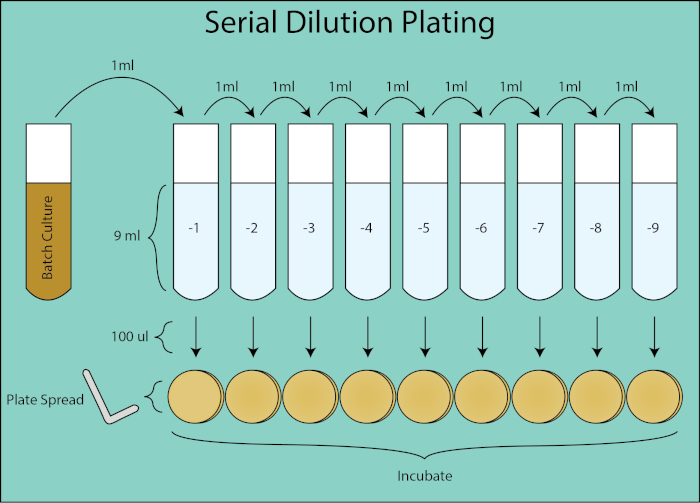
איור 2. שרטוט ציפוי דילול סדרתי. זרימה כללית ל ציפוי דילול מתרבות האצווה. תרבות האצווה מדוללת באופן סדרתי 1:10 על-ידי העברת 1 מ”ל של הדילול הקודם לצינור הבא המכיל 9 מ”ל PBS. מכל צינור דילול, 100 μl הוא מפוזר מצופה באמצעות מפיץ צלחת שהוא דילול נוסף של 1:10 כפי שהוא 1/10את הנפח של נפח 1 מ”ל בעת חישוב CFU / mL. צלחות הם דגירה והספירה פעם מושבות כלנית לגדול על הצלחות.

לאחר מכן הלוחות דוגרים בן לילה ומושבות כלונסאות נפרמות. לוח הדילול שצמח 30-300 מושבות משמש לחישוב CFU / mL עבור נקודת הזמן הנתונה (4, 5). וריאציה סטוכסטית בספירת המושבות מתחת לגיל 30 כפופה לשגיאה גדולה יותר בחישוב של CFU / mL וספירת מושבות הגדולות מ -300 ניתן להמעיט בערכן עקב צפיפות וחפיפה במושבה. באמצעות גורם הדילול עבור הצלחת הנתונה, ניתן לחשב את ה- CFU של תרבות האצווה עבור כל נקודת זמן.

צפיפות אופטית נותנת קירוב מיידי של ספירת תאים חיידקיים נמדד באמצעות ספקטרופוטומטר. הצפיפות האופטית היא מדד לספיגה של חלקיקי אור העוברים דרך 1 ס”מ של תרבות ומזוהים על ידי חיישן פוטודיודה (6). הצפיפות האופטית של תרבית נמדדת ביחס לתקשורת ריקה ומתגברת ככל שצפיפות החיידקים גדלה. עבור תאים חיידקיים, אורך גל של 600 ננומטר (OD600) משמש בדרך כלל בעת מדידת צפיפות אופטית (4). על ידי יצירת עקומה סטנדרטית הנוגעת ליחידות יצירת מושבה וצפיפות אופטית, ניתן להשתמש במדידת הצפיפות האופטית כדי להעריך בקלות את ספירת תאי החיידקים של תרבית אצווה. עם זאת, מערכת יחסים זו מתחילה להידרדר כבר 0.3 OD600 כמו תאים מתחילים לשנות צורה לצבור מוצרים חוץ תאיים במדיה, המשפיעים על קריאת הצפיפות האופטית כפי שהוא מתייחס CFU (7). שגיאה זו הופכת בולטת יותר במהלך שלבי נייח ומוות.

כאן, Escherichia coli גדל מרק לוריא-ברטאני (LB) ב 37 מעלות צלזיוס במהלך 30 שעות (7). הן עקומות צמיחה CFU / mL והן עקומות צמיחה בצפיפות אופטית נוצרו, כמו גם העקומה הסטנדרטית הנוגעת לצפיפות אופטית ל- CFU.

Figure 3
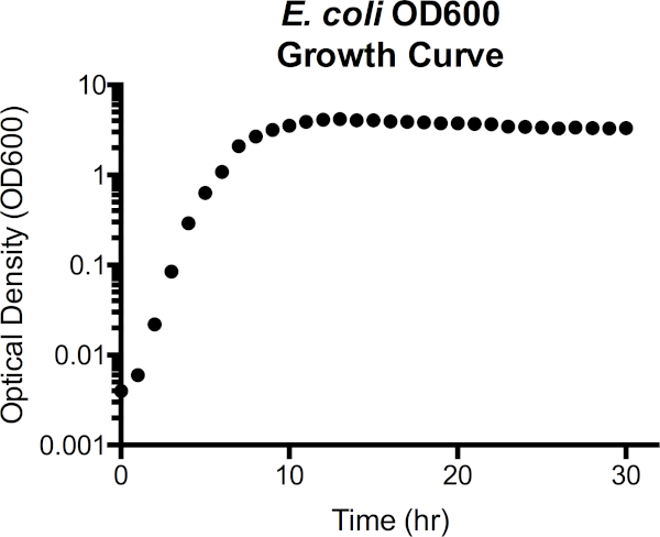
איור 3. Escherichia coli צפיפות אופטית באורך גל 600 ננומטר (OD600) עקומת גדילה. ערכי צפיפות אופטית נלקחו ישירות מהספקטרופוטומטר לאחר ריקון עם מדיית LB סטרילית. ערכי OD600 הגדולים מ- 1.0 דוללו 1:10 על-ידי שילוב של תרבות 100 מיקרול עם 900 μl LB טרי, נמדד שוב ולאחר מכן הוכפל ב- 10 כדי להשיג את הערך OD600. שלב זה נלקח כמו הדיוק במדידה של ספקטרופוטומטר מופחת בצפיפות תאים גבוהה. מהעיקול, שלב ההשהיה משתרע על 1h של צמיחה, מעברים לשלב מעריכי מ 2h ל 7h, ואז מתחיל לרמה, נכנס לשלב נייח. שלב המוות אינו מעבר מוחלט, עם זאת, כמו צפיפות אופטית בהדרגה מתחיל לרדת לאחר 15h.

Figure 4
איור 4. עקומת הצמיחה של מושבת Escherichia coli ליצירת יחידה למיליליטר (CFU/mL). ערכי CFU/mL עבור כל נקודת זמן חושבו מתוך לוח הדילול שהכיל 30-300 מושבות. מהעיקול, שלב ההשהיה משתרע על פני כ-2h של צמיחה, מעברים לשלב מעריכי מ-2h ל-7h, ואז מתחילים לרמה, נכנסים לשלב נייח. שלב המוות אינו מעבר מוחלט, עם זאת, כמו CFU / mL בהדרגה מתחיל לרדת לאחר 15 שעות משיא של 2 x 10⁹ לכ 5 x 10⁸ ב 30 שעות.

Figure 5
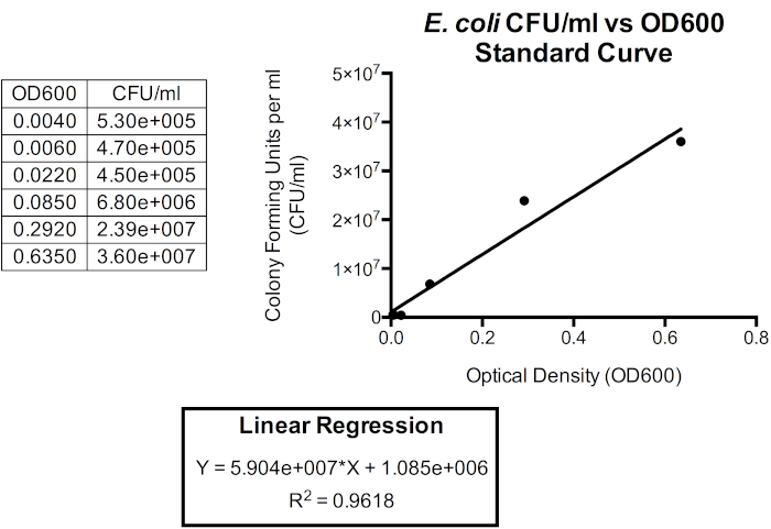
איור 5. עקומת תקינה עבור CFU/mL לעומת OD600. רגרסיה ליניארית יכולה לשמש כדי לקשר יחידות אלה, כך צפיפות אופטית עשויה לשמש צפיפות תאים חיידקי משוער. ניתן להשתמש בצפיפות אופטית כדי לספק קירוב מיידי של CFU / mL של תרבות האצווה. כאן, רק שש נקודות הזמן הראשונות מותוותות מכיוון שהקשר בין OD600 ל- CFU/mL פחות מדויק מעבר ל- 1.0 OD600 כאשר צורת התא ומוצרים חוץ-תאיים מתחילים להצטבר כאשר החיידקים נכנסים לשלב נייח, המתרחש זמן קצר לאחר שהגיעו ל- 1.0 OD600. שינויים בצורת התא ובמוצרים חוץ תאיים במדיה משפיעים על קריאת הצפיפות האופטית ולכן הקשר בין צפיפות אופטית למספר החיידקים בתרבות מושפע גם הוא.

זמן ההכפלה נקבע גם הוא להיות 15 דקות ו -19 שניות. מנתונים אלה, ניתן לדמיין את יכולת הצמיחה ב- LB עבור E. coli ולהשתמש בה להשוואה בין מדיה או חיידקים שונים.

Procedure

1. הגדרת חומרי מעבדה נדרשים: מדיה נוזלית, מדיית אגר מוצקה, צלוחיות ארלנמאייר, מברכות 15 מ”ל, תמיסת מלח חוצצת פוספט (PBS), מפיץ תאים חיידקיים, 70% אתנול וספטרופיוטומטר. יש לעקר את כל הפתרונות וכלי הזכוכית לפני השימוש. הכן את תחנת העבודה על ידי עיקור עם 70% אתנול. לעבוד ליד מבער בונ?…

Results

Plots of colony forming units and optical density are two ways to visualize growth kinetics. By determining the relationship between CFU/mL and OD600, the optical density plot also provides an estimate of CFU/mL over time. Conditions that result in the shortest doubling time are considered optimal for growth of the given bacteria.

Applications and Summary

Growth curves are valuable for understanding the growth kinetics and physiology of bacteria. They allow us to determine how bacteria respond in variable growth conditions as well as define the optimal growth parameters for a given bacterium. Colony forming unit and optical density plots both contain valuable information depicting the duration of lag phase, maximum cell density reached, and allowing for the calculation of bacterial doubling time. Growth curves also allow for comparison between different bacteria under the same growth conditions. Additionally, optical density provides a means of standardizing initial inoculums, enhancing consistency in other experiments.

Determining which approach to use when designing a growth curve experiment requires consideration. As the preferred method for generating growth curves, colony forming unit plots more accurately reflect the viable cell counts in batch culture. Colony forming unit plots also allow for measuring bacterial growth in conditions that would otherwise interfere with an optical density measurement. However, it is a more time consuming process, requiring extensive use of reagents, and must be performed manually. Optical density plots are less accurate and provide only an estimate of the colony forming units, requiring a standard curve to be generated for each unique bacteria. Optical density is primarily used for its convenience as it is far less time consuming and does not require many reagents to perform. What is most attractive to optical density, is that spectrophotometric incubators can automatically generate growth curves, vastly increasing the number of culture conditions that can be tested at once and eliminating the need to constantly attend the culture.

References

  1. R. E. Buchanan. 1918. Life Phases in a Bacterial Culture. J Infect Dis 23:109-125.
  2. CAMPBELL A. 1957. Synchronization of cell division. Bacteriol Rev 21:263-72.
  3. Wang P, Robert L, Pelletier J, Dang WL, Taddei F, Wright A, Jun S. 2010. Robust growth of Escherichia coli. Curr Biol 20:1099-103.
  4. Goldman E, Green LH. 2015. Practical Handbook of Microbiology, Third Edition. CRC Press.
  5. Ben-David A, Davidson CE. 2014. Estimation method for serial dilution experiments. J Microbiol Methods 107:214-221.
  6. Koch AL. 1968. Theory of the angular dependence of light scattered by bacteria and similar-sized biological objects. J Theor Biol 18:133-156.
  7. Sezonov G, Joseleau-Petit D, D'Ari R. 2007. Escherichia coli physiology in Luria-Bertani broth. J Bacteriol 189:8746-9.

Transcript

Bacteria reproduce through a process called cell division, which results in two identical daughter cells. If the growth conditions are favorable, bacterial populations will grow exponentially.

Bacterial growth curves plot the amount of bacteria in a culture as a function of time. A typical growth curve progresses through four stages: lag phase, exponential phase, stationary phase, and death phase. The lag phase is the time it takes for bacteria to reach a state where they can grow and divide quickly. After this, the bacteria transition to the exponential phase, characterized by rapid cell growth and division. The rate of exponential growth of the bacterial culture during this phase can be expressed as the doubling time, the fastest rate at which bacteria can reproduce under specific conditions. The stationary phase comes next, where bacterial cell growth plateaus and the growth and death rates even out due to environmental nutrient depletion. Finally, the bacteria enter the death phase. This is where bacterial growth declines sharply and severe nutrient depletion leads to the lysing of cells.

Two techniques can be used to quantify the amount of bacteria present in a culture and plot a growth curve. The first of these is via colony forming units, or CFUs. To obtain CFUs a one to ten series of nine dilutions is performed at regular time points. The first of these dilutions, negative one in this example, contains 9mL of PBS and 1mL of the bacterial culture. Resulting in a 1:10 dilution factor. Then, 1mL of this solution is transferred to the next tube, negative two, resulting in a 1:100 dilution factor. This process continues through the last tube, negative nine, resulting in a final dilution factor of 1:1 billion. After this, 100 microliters of each dilution is plated. The plates are then incubated and the clonal colonies are counted. The dilution plate for a given time point that grows between 30 and 300 colonies is used to calculate the CFUs per milliliter for that time point.

The second common method of measuring bacterial concentration is the optical density. The optical density of a culture can be measured instantly, in relation a media blank, with a spectrophotometer. Typically a wave length of 600 nanometers, also referred to as OD600, is used for these measurements, which increase as cell density increases. While optical density is less precise than CFUs, it is convenient because it can be obtained instantaneously and requires relatively few reagents. Both techniques can be used together to create a standard curve that more accurately approximates the bacterial cell count of a culture. In this video, you will learn how to obtain CFUs and OD600 measurements from timed serial dilutions of E. coli. Then, two growth curves using the CFU and OD600 measurements, respectively, will be plotted before being related by a standard curve.

When working with bacteria, it is important to use the appropriate personal protective equipment such as a lab coat and gloves and to observe proper aseptic technique.

After this, sterilize the work station with 70% ethanol. First, prepare the LB broth and LB solid agar media in separate autoclaveable bottles. After partially closing the caps of the bottles, sterilize the media in an autoclave set to 121 degrees Celsius for 35 minutes. Next, allow the agar media to cool in a water bath set to 50 degrees Celsius for 30 minutes. Once cooled, pour 20 to 25 mL into each Petri dish. After this, allow the plates to set for 24 hours at room temperature.

To prepare the single colony isolates that will later be used to produce a liquid bacterial culture, use previously frozen stock and proper streak plating technique to streak E. coli for isolation on LB agar. Incubate the dish at 37 degree Celsius overnight. After this, cool a flame sterilized inoculation loop on the agar before selecting a single colony from the streaked plate. Inoculate 4 mL of liquid media in a 15 mL test tube. Then, grow the E. coli at 37 degrees Celsius overnight with shaking at 210 rpm.

To set up the 1:1000 volume of bacterial culture that will be used in the growth curve, first obtain an autoclaved 500 mL Erlenmeyer flask. Then, use a 50 mL serological pipette to transfer 100 mL of sterile media to the flask. Next, label nine 15 ml test tubes consecutively as one through nine. These numbers correspond to the dilution factor that will be used to calculate the colony forming unit, or CFU. Then, add 9 mL of 1X PBS to each tube. After this, label the prepared agar plates with the corresponding time points and dilution factors that will be grown. In this example with E. coli, after the starting time point, time points are taken once every hour. Using the previously prepared overnight liquid E. coli culture, inoculate the media in the autoclave 500 mL Erlenmeyer flask with 1:1000 volume of culture. Swirl the media to evenly distribute the bacteria.

After blanking a spectrophotometer, clean the cuvette with a lint-free wipe. Next, dispense 1 mL of the culture into the cuvette and place it into the spectrophotometer to obtain the optical density of the culture at time point zero. Then, grow the E. coli at 37 degrees Celsius with shaking at 210 rpm. At each time point after time point zero, withdraw another 1 mL of bacterial culture from the flask and repeat the optical density measurement. If the optical density reading is greater than 1.0, dilute 100 microliters of bacterial culture with 900 microliters of fresh media and then measure the optical density once more. This value can be multiplied by 10 for the OD 600 measurement.

To obtain the colony forming unit measurement for each time point, withdraw an additional 1 mL of bacterial culture from the flask at each time point. Dispense the bacterial culture into the negative one test tube and vortex to mix. Then, perform the dilution series by first transferring 1 mL from the negative one tube into the negative two tube and vortex to mix. Transfer 1 mL from the negative two tube into the negative three tube and vortex to mix. Continue this serial transfer down all the dilution tubes to the negative nine tube. Dispense 100 microliters of cell suspension onto the correspondingly labeled plate for each dilution. For every dilution, sterilize a cell spreader in ethanol, pass it through a Bunsen burner flame, and cool it by touching the surface of the agar away from the inoculate. Then, use the cell spreader to spread the cell suspension until the surface of the agar plate becomes dry. Incubate the plates upside down at 37 degrees Celsius. Once visible colonies arise, count the number of bacterial colonies on each plate. Record these values and their associated dilution factors for each plate at each time point.

To create an OD 600 growth curve, after ensuring all the data points are entered correctly into a table, select all of the time points and their corresponding data. To generate a colony forming unit growth curve plot, choose the dilution plate where the colony counts fell within the range 30 to 300 bacteria for each time point. Multiply the colony count number by the dilution factor, and then by ten. This is because the 100 microliters spread is considered an additional 1:10 dilution when calculating colony forming units per milliliter. After this, plot the colony forming units versus time on a semi-log scale.

These plots produced with OD 600 and CFU measurements, respectively, can provide valuable information on E. coli growth kinetics. The optical density and colony forming units can be related, so that CFUs per milliliter can be estimated from OD 600 measurements, saving time and materials in future experiments.

To do this, plot the colony forming units against the optical density on a linear scale for OD 600 readings less than or equal to 1. 0. After this, generate a linear regression trend line in Y = MX + B format, where M is the slope and B is the y-intercept. Right click on the data points and select add trend line and linear. Then, check the box to display the equation on the chart and display the R squared value on the chart. The R squared value is the statistical measurement of how closely the data matched the fitted regression line. In this example, the first 6 time points are plotted with OD 600 on the x axis and CFUs per milliliter on the y axis. In future experiments with the same growth conditions, these slope and y-intercept values can be plugged into this equation to estimate CFUs from OD 600 readings. Next, look at the colony forming unit growth curve plot. During the exponential phase, identify two time points with the steepest slope between them. To calculate the doubling time, first calculate the change in time between the selected time points. Then, calculate the change in generations using the equation shown here. Here, lower case b is the number of bacteria at time point three and upper case B is the number of bacteria at time point two. Finally, divide the change in time by the change in generations. In this example, the doubling time is 0. 26 hours or 15 minutes and 19 seconds. Comparing doubling times across different experimental treatment allows us to identify the best growth conditions for a certain bacterial species. Therefore, the treatment with the lowest doubling time will be most optimal of the conditions tested.

Tags

Cite This
JoVE Science Education Database. JoVE Science Education. Growth Curves: Generating Growth Curves Using Colony Forming Units and Optical Density Measurements. JoVE, Cambridge, MA, (2023).