Bacteria reproduce through a process called cell division, which results in two identical daughter cells. If the growth conditions are favorable, bacterial populations will grow exponentially.
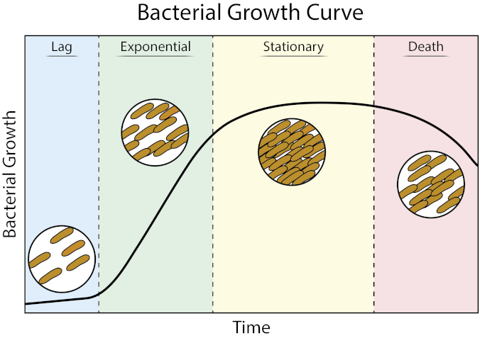
Bacterial growth curves plot the amount of bacteria in a culture as a function of time. A typical growth curve progresses through four stages: lag phase, exponential phase, stationary phase, and death phase. The lag phase is the time it takes for bacteria to reach a state where they can grow and divide quickly. After this, the bacteria transition to the exponential phase, characterized by rapid cell growth and division. The rate of exponential growth of the bacterial culture during this phase can be expressed as the doubling time, the fastest rate at which bacteria can reproduce under specific conditions. The stationary phase comes next, where bacterial cell growth plateaus and the growth and death rates even out due to environmental nutrient depletion. Finally, the bacteria enter the death phase. This is where bacterial growth declines sharply and severe nutrient depletion leads to the lysing of cells.
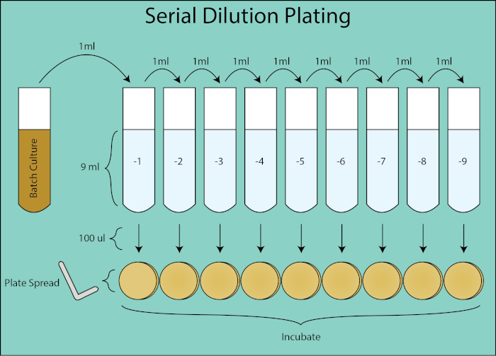
Two techniques can be used to quantify the amount of bacteria present in a culture and plot a growth curve. The first of these is via colony forming units, or CFUs. To obtain CFUs a one to ten series of nine dilutions is performed at regular time points. The first of these dilutions, negative one in this example, contains 9mL of PBS and 1mL of the bacterial culture. Resulting in a 1:10 dilution factor. Then, 1mL of this solution is transferred to the next tube, negative two, resulting in a 1:100 dilution factor. This process continues through the last tube, negative nine, resulting in a final dilution factor of 1:1 billion. After this, 100 microliters of each dilution is plated. The plates are then incubated and the clonal colonies are counted. The dilution plate for a given time point that grows between 30 and 300 colonies is used to calculate the CFUs per milliliter for that time point.
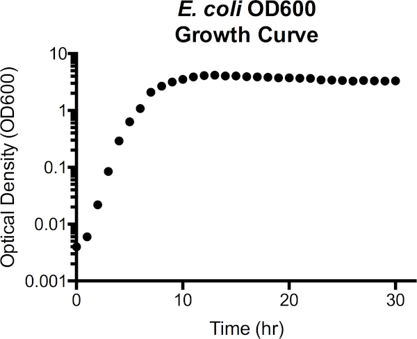
The second common method of measuring bacterial concentration is the optical density. The optical density of a culture can be measured instantly, in relation a media blank, with a spectrophotometer. Typically a wave length of 600 nanometers, also referred to as OD600, is used for these measurements, which increase as cell density increases. While optical density is less precise than CFUs, it is convenient because it can be obtained instantaneously and requires relatively few reagents. Both techniques can be used together to create a standard curve that more accurately approximates the bacterial cell count of a culture. In this video, you will learn how to obtain CFUs and OD600 measurements from timed serial dilutions of E. coli. Then, two growth curves using the CFU and OD600 measurements, respectively, will be plotted before being related by a standard curve.
When working with bacteria, it is important to use the appropriate personal protective equipment such as a lab coat and gloves and to observe proper aseptic technique.
After this, sterilize the work station with 70% ethanol. First, prepare the LB broth and LB solid agar media in separate autoclaveable bottles. After partially closing the caps of the bottles, sterilize the media in an autoclave set to 121 degrees Celsius for 35 minutes. Next, allow the agar media to cool in a water bath set to 50 degrees Celsius for 30 minutes. Once cooled, pour 20 to 25 mL into each Petri dish. After this, allow the plates to set for 24 hours at room temperature.
To prepare the single colony isolates that will later be used to produce a liquid bacterial culture, use previously frozen stock and proper streak plating technique to streak E. coli for isolation on LB agar. Incubate the dish at 37 degree Celsius overnight. After this, cool a flame sterilized inoculation loop on the agar before selecting a single colony from the streaked plate. Inoculate 4 mL of liquid media in a 15 mL test tube. Then, grow the E. coli at 37 degrees Celsius overnight with shaking at 210 rpm.
To set up the 1:1000 volume of bacterial culture that will be used in the growth curve, first obtain an autoclaved 500 mL Erlenmeyer flask. Then, use a 50 mL serological pipette to transfer 100 mL of sterile media to the flask. Next, label nine 15 ml test tubes consecutively as one through nine. These numbers correspond to the dilution factor that will be used to calculate the colony forming unit, or CFU. Then, add 9 mL of 1X PBS to each tube. After this, label the prepared agar plates with the corresponding time points and dilution factors that will be grown. In this example with E. coli, after the starting time point, time points are taken once every hour. Using the previously prepared overnight liquid E. coli culture, inoculate the media in the autoclave 500 mL Erlenmeyer flask with 1:1000 volume of culture. Swirl the media to evenly distribute the bacteria.
After blanking a spectrophotometer, clean the cuvette with a lint-free wipe. Next, dispense 1 mL of the culture into the cuvette and place it into the spectrophotometer to obtain the optical density of the culture at time point zero. Then, grow the E. coli at 37 degrees Celsius with shaking at 210 rpm. At each time point after time point zero, withdraw another 1 mL of bacterial culture from the flask and repeat the optical density measurement. If the optical density reading is greater than 1.0, dilute 100 microliters of bacterial culture with 900 microliters of fresh media and then measure the optical density once more. This value can be multiplied by 10 for the OD 600 measurement.
To obtain the colony forming unit measurement for each time point, withdraw an additional 1 mL of bacterial culture from the flask at each time point. Dispense the bacterial culture into the negative one test tube and vortex to mix. Then, perform the dilution series by first transferring 1 mL from the negative one tube into the negative two tube and vortex to mix. Transfer 1 mL from the negative two tube into the negative three tube and vortex to mix. Continue this serial transfer down all the dilution tubes to the negative nine tube. Dispense 100 microliters of cell suspension onto the correspondingly labeled plate for each dilution. For every dilution, sterilize a cell spreader in ethanol, pass it through a Bunsen burner flame, and cool it by touching the surface of the agar away from the inoculate. Then, use the cell spreader to spread the cell suspension until the surface of the agar plate becomes dry. Incubate the plates upside down at 37 degrees Celsius. Once visible colonies arise, count the number of bacterial colonies on each plate. Record these values and their associated dilution factors for each plate at each time point.
To create an OD 600 growth curve, after ensuring all the data points are entered correctly into a table, select all of the time points and their corresponding data. To generate a colony forming unit growth curve plot, choose the dilution plate where the colony counts fell within the range 30 to 300 bacteria for each time point. Multiply the colony count number by the dilution factor, and then by ten. This is because the 100 microliters spread is considered an additional 1:10 dilution when calculating colony forming units per milliliter. After this, plot the colony forming units versus time on a semi-log scale.
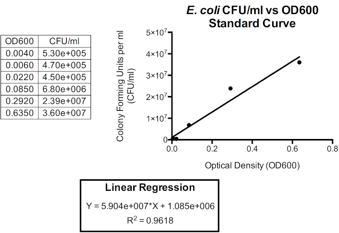
These plots produced with OD 600 and CFU measurements, respectively, can provide valuable information on E. coli growth kinetics. The optical density and colony forming units can be related, so that CFUs per milliliter can be estimated from OD 600 measurements, saving time and materials in future experiments.
To do this, plot the colony forming units against the optical density on a linear scale for OD 600 readings less than or equal to 1. 0. After this, generate a linear regression trend line in Y = MX + B format, where M is the slope and B is the y-intercept. Right click on the data points and select add trend line and linear. Then, check the box to display the equation on the chart and display the R squared value on the chart. The R squared value is the statistical measurement of how closely the data matched the fitted regression line. In this example, the first 6 time points are plotted with OD 600 on the x axis and CFUs per milliliter on the y axis. In future experiments with the same growth conditions, these slope and y-intercept values can be plugged into this equation to estimate CFUs from OD 600 readings. Next, look at the colony forming unit growth curve plot. During the exponential phase, identify two time points with the steepest slope between them. To calculate the doubling time, first calculate the change in time between the selected time points. Then, calculate the change in generations using the equation shown here. Here, lower case b is the number of bacteria at time point three and upper case B is the number of bacteria at time point two. Finally, divide the change in time by the change in generations. In this example, the doubling time is 0. 26 hours or 15 minutes and 19 seconds. Comparing doubling times across different experimental treatment allows us to identify the best growth conditions for a certain bacterial species. Therefore, the treatment with the lowest doubling time will be most optimal of the conditions tested.