A method to quantify the orofacial size and shape of Xenopus laevis embryos has been developed. In this protocol, traditional size measurements are combined with geometric morphometrics to allow for more sophisticated analyses of orofacial development and defects.
Xenopus has become an important tool for dissecting the mechanisms governing craniofacial development and defects. A method to quantify orofacial development will allow for more rigorous analysis of orofacial phenotypes upon abrogation with substances that can genetically or molecularly manipulate gene expression or protein function. Using two dimensional images of the embryonic heads, traditional size dimensions-such as orofacial width, height and area- are measured. In addition, a roundness measure of the embryonic mouth opening is used to describe the shape of the mouth. Geometric morphometrics of these two dimensional images is also performed to provide a more sophisticated view of changes in the shape of the orofacial region. Landmarks are assigned to specific points in the orofacial region and coordinates are created. A principle component analysis is used to reduce landmark coordinates to principle components that then discriminate the treatment groups. These results are displayed as a scatter plot in which individuals with similar orofacial shapes cluster together. It is also useful to perform a discriminant function analysis, which statistically compares the positions of the landmarks between two treatment groups. This analysis is displayed on a transformation grid where changes in landmark position are viewed as vectors. A grid is superimposed on these vectors so that a warping pattern is displayed to show where significant landmark positions have changed. Shape changes in the discriminant function analysis are based on a statistical measure, and therefore can be evaluated by a p-value. This analysis is simple and accessible, requiring only a stereoscope and freeware software, and thus will be a valuable research and teaching resource.
Among the most prevalent and devastating types of human birth defects are those affecting the mouth and face, such as orofacial clefts1. Children with malformed orofacial structures undergo multiple surgeries throughout their lifetime and struggle with facial disfigurements, speech, hearing and eating problems. Therefore, facilitating new research in cranio- and orofacial development is paramount to prevention and treatment of these types of birth defects in humans. Xenopus laevis has emerged as a new tool for dissecting the mechanisms governing craniofacial development (some examples include2,3,4-11). Therefore, a quantitative method to analyze size and shape changes during development of the head and face of this species could be very powerful 3.
Here, we present such a method; combining traditional size measurements with geometric morphometrics adapted from a Xenopus study12 and a wealth of studies analyzing human facial form13-15. The goal of this protocol is to allow researchers to quantify facial size and shapes to distinguish between different orofacial phenotypes during normal and abnormal development. This analysis will allow for better differentiation between subtle craniofacial defects such as those arising from synergistic effects of genes and/or environmental factors. Additionally, this quantification method could also reveal even slight improvement or rescue of an orofacial defect. This therefore makes it a useful guide in analyzing potential therapeutics.
The combination of facial measurements and geometric morphometrics that we present here allows for a more comprehensive statistical analysis of both size and shape of the orofacial region than current protocols which largely utilize only one or the other15-18. Further, we present a simple way to assess both the medial and lateral planes of the face without requiring sophisticated three-dimensional imaging equipment used in current studies13,19.
We demonstrate this protocol on Xenopus laevis embryos treated with a retinoic acid receptor inhibitor that induces abnormal orofacial development and a median cleft palate2,3. Quantification of the dimensions and shape of the orofacial region in these embryos has revealed changes in the midface that is analogous to humans with similar palatal clefts and mouse models 20,21. However, this protocol can be utilized to assess the effects of other compounds on orofacial development such as natural substances, herbicides, or proteins such as growth factors. Further, orofacial size and shape changes arising from perturbation of gene expression via loss or gain of function experiments (using antisense morpholinos or Crispers/Talens) can also be quantified using this protocol. Finally, we developed this method specifically to assess Xenopus morphology; however, it is easily modified for analysis of any vertebrate. Other applications could also include using this protocol for comparing closely related species for evolutionary or ecological studies. While the example we provide here utilizes this protocol to describe analysis of the orofacial region, it could easily be modified for analysis of other regions, organs, or structures.
This orofacial quantification protocol will become a valuable resource for the research community, as well as an excellent teaching tool for undergraduate students as a video demonstration.
All experiments performed using Xenopus laevis have been approved by IACUC (protocol #AD20261) .
1. Preparing Reagents and Required Materials
2. Xenopus laevis Embryo Culture and Inhibitor Treatments
3. Photographing the Orofacial Region of Xenopus Tadpoles
4. Measuring and Analyzing Facial Size Dimensions in Xenopus Tadpoles
5. Quantitative Analysis of Orofacial Shape and Morphometrics
Here, a quantitative analysis of orofacial size and shape was demonstrated to compare embryos treated with a retinoic acid receptor inhibitor (RAR inhibitor) to untreated controls. Embryos were treated with a 1 μM concentration of this chemical inhibitor from stage 24 to 30 (26-35 hpf), washed out, and fixed at stage 42 (82 hpf). They were then processed and analyzed as described in the protocol. Results are original data, but consistent with observations in previous publications2,3. Control embryos were treated with the vehicle, DMSO, and developed normally (Figure 7Ai,ii). Embryos treated with a 1 μM concentration of the RAR inhibitor showed slight narrowing of the face, eye anomalies, and a malformed embryonic mouth opening that was more triangular shaped (Figure 7Aiii,iv).
First, traditional orofacial dimensions were measured and are summarized in Figure 7B. Statistical significance was determined by performing a Student’s t-test assuming unequal variance between inhibitor treated embryos and controls for each measurement. We found that both snout length and face width were significantly decreased in RAR inhibitor treated embryos compared to controls (p-values = 0.0062 and 0.0058, respectively; Figure 7Bi,ii). While face height and mouth roundness were significantly increased (p-values = 3.7772 x 10⁻⁶, 1.4812 x 10⁻⁷), mouth width was significantly decreased (p-value = 2.5175 x 10⁻¹⁰; Figure 7Biii-v).The results showed no significant difference in the overall orofacial area between the two groups (p-value = 0.3754; Figure 7Bvi). These data show that loss of retinoic acid signaling at a specific time in development results in a shorter snout, slight narrowing of the midface region, and malformation of the embryonic mouth opening.
To provide a sophisticated view of the shape changes of the embryonic orofacial region in response to reduced retinoic acid signals, we next utilized geometric morphometric analyses. After identifying and aligning orofacial landmarks using morphometric analysis software, we then examined the variance within each group via principal component analysis (PCA). When the first two principal components were plotted against each other, RAR inhibitor treated embryos were clearly distinguished from controls along the PC1 axis (Figure 7C). This test also showed the outliers in the sample set- illustrated by two inhibitor treated embryos that did not cluster with the rest of the group (Figure 7C, arrows).
Next, the statistical differences in the shape of the orofacial region between RAR inhibitor treated embryos and controls were assessed and visualized by performing a discriminant function analysis (DFA). The Procrustes distance between the two groups was significantly different (distance = 0.2665, p-value < 0.0001, Figure 7D), indicating a change in orofacial shape when retinoic acid signaling is disrupted. Indeed, dramatic shifts in the position of lateral landmarks in the orofacial region indicate a narrowing of the face shape respective to the height in inhibitor treated embryos (Figure 7D). In addition, the slight outward shift in position of the nasal landmarks (Figure 7D, arrows) reveals the abnormality in nostril position in these embryos that is consistent with decreased outgrowth of the snout. The shifts in landmarks that define the edges of the mouth opening show position changes that reflect the formation of a triangular shaped mouth opening that is consistent with the median cleft reported in our previous studies 2,3. In addition to vector shifts, the warping pattern of the transformation grid also illustrates shape changes in the orofacial region. Warping in the midface region is consistent with the midface hypoplasia and overall facial narrowing seen in embryos with decreased retinoic acid signals (Figure 7D).
The results of the discriminant function analysis (DFA) show shape changes that were consistent with our qualitative analysis, as well as revealing some changes that were not adequately captured by traditional size measurements alone. For instance, while the orofacial area was not significantly different between controls and inhibitor treated embryos (Figure 7Bvi), the DFA transformation grid revealed dramatic changes in this region consistent with the facial narrowing seen in inhibitor treated embryos (Figure 7A,D). Further, the warping pattern and landmark shifts of the mouth opening, coupled with the significant change we saw in mouth roundness, illustrate the malformation of the mouth opening shape in inhibitor treated embryos. In summary, a combination of traditional measurements of facial dimensions and geometric morphometric analysis illustrates the changes in shape and size of the orofacial region when retinoic acid signals are disrupted.
Figure 1. Required materials. (A) Tools for data analysis. (i) 24-well plate, (ii) standard disposable transfer pipette, (iii) Dumont #5 Inox forceps, (iv) clay-lined Petri dish, (v) straight teasing needle, (vi) glass pipette tool, (vii) sterile, disposable scalpel. (B) Preparation of the clay-lined dish. (i) A straight teasing needle is used to draw horizontal lines in the clay. (ii) A glass pipette tool is used to make circular depressions along each row. (iii) The dish is filled with PBT for imaging.
Figure 2. In vitro fertilization and culture of Xenopus eggs. (A) Following HCG injection, adult Xenopus laevis females are induced to lay eggs. (B) Eggs are collected in high salt MBS, fertilized with testes extracted from a male, and cultured using standard methods. (C) Embryos are transferred to a 24-well dish containing 0.1x MBS using a standard, disposable transfer pipette. (D) A calibrated pipette-man is used to measure 1 ml into an empty well, and a marker is used to demarcate this level on the outside of all wells containing embryos (inset). 0.1x MBS is then added or taken away so that it is level with this mark.
Figure 3. Preparation of embryo heads for imaging. (A) Diagram of the two incisions required to remove heads, solid black lines. Scale bar = 400 μm. (B) The first incision is made at the posterior end of the gut to remove the tail and release pressure from the scalpel. Scale bar = 400 μm. (C) The second incision is made at the anterior end of the gut, near the heart, to completely sever the head. Scale bar = 400 μm. (D) Frontal views of row of embryo heads positioned in clay. Scale bar = 650 µm. (E) Lateral views of row of embryo heads position in clay. Scale bar = 500 µm cg: cement gland.
Figure 4. Traditional size measurements of orofacial dimensions. (A) Face width. Arrows indicate the points where the ventral portion of the eye meets the periphery of the face. Red line is the face width, measured as the distance between these points. Scale bar = 210 µM. (B) Face Height. White lines are guides drawn prior to measurement at the dorsal edge of the eyes and the dorsal edge of the cement gland. Red line is the face height, measured as the distance between these two guides at the midline of the face. Scale bar = 210 µM. (C) Orofacial area. White lines are guides drawn prior to measurement. (a) Point where the bottom guide meets the ventral edge of the left eye. Red line shows the tracing around the left eye. (b) Point where the dorsal edge of the eye meets the top guide. Blue line shows the dorsal boundary of orofacial area, traced along the top guide at the dorsal edge of the eyes. (c) Point where the top guide meets the right facial periphery. Green line shows the tracing around the right eye. (d) Point where the ventral edge of the right eye meets the bottom guide. Yellow line shows ventral boundary of orofacial area, traced along the bottom guide at the dorsal edge of the cement gland. Scale bar = 210 µM. (D) Snout length. White line is the anterior edge of the eye and is drawn as a guide prior to measurement. Red line is snout length, measured from this line to the point where the dorsal edge of the cement gland meets the lateral periphery of the face. Scale bar = 300 µM. (E) Mouth width. Arrows are the points where the dorsal and ventral lips meet. The red line is the mouth width, measured as the distance between these two points. Scale bar = 200 µM. (F) Mouth roundness. The perimeter of the mouth opening is traced and shown in red. cg: cement gland. Scale bar = 200 µM.
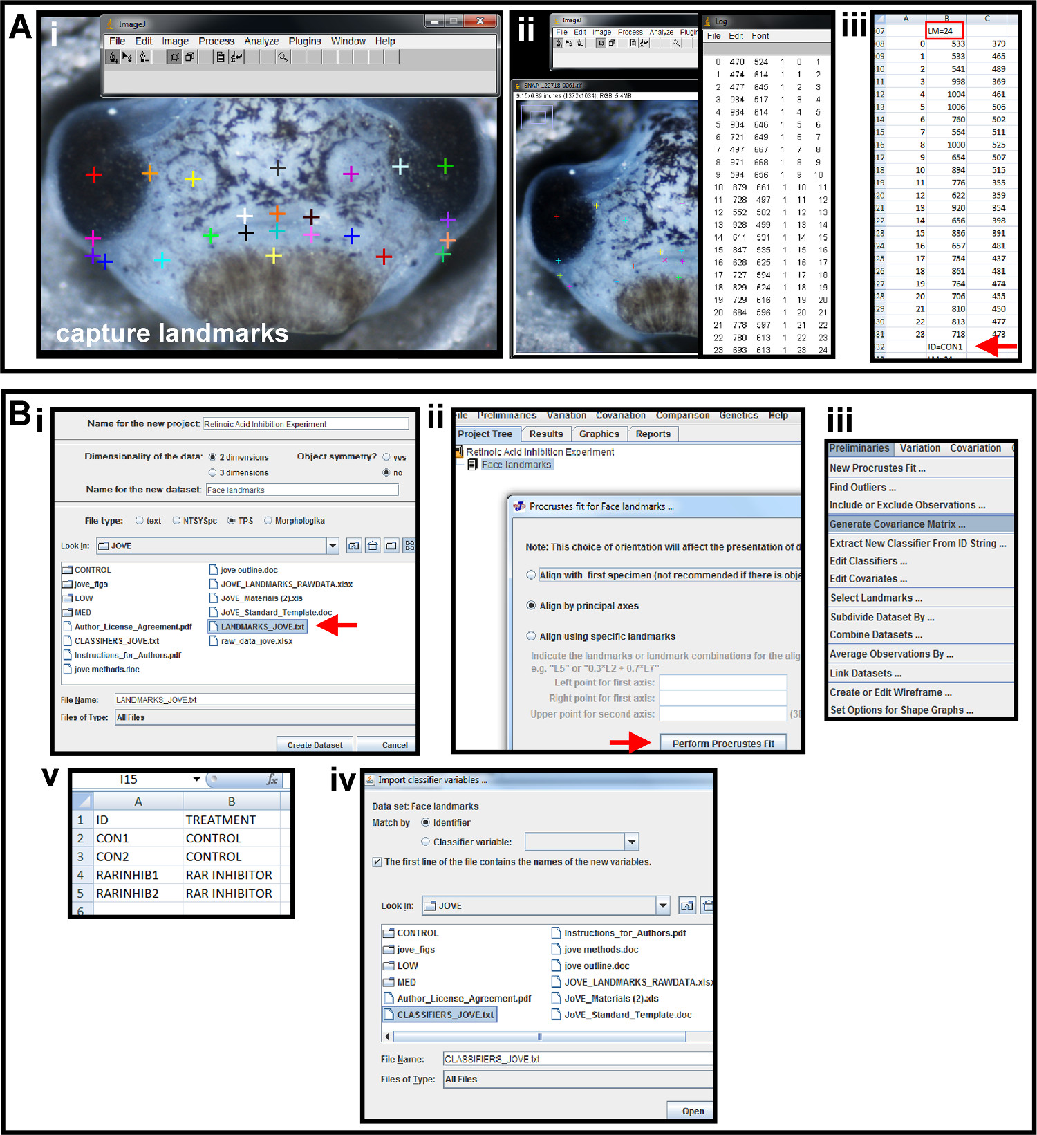
Figure 5. Capturing landmarks and preliminaries for geometric morphometric analysis. (A) Using photo-editing software and a spreadsheet program to place landmarks and capture coordinates. (i) Multicolored crosses are the landmarks placed on the image using the Add points tool in ImageJ to represent the shape of the orofacial region. (ii) Landmark data is displayed by using the Display Results Tool. (iii) Landmark data is copied and pasted into a spreadsheet. Above the second column is a header identifying the number of landmarks and denoted by "LM=24" (red box). Below the second column of data, the sample is given a unique name and denoted by "ID=CON1" (red arrow). This is repeated for all images in a sample set and the data is saved as a text file. (B) Preliminary data analysis in a geometric morphometric software program. (i) The text file created in from the photo-editing software is imported into the morphometric program, MorphoJ, as a TPS file. File is indicated by red arrow. (ii) Landmark coordinate data is aligned by Procrustes fit by principal axes. Red arrow indicates execution of alignment. (iii) A covariance matrix of Procrustes fit landmarks is generated in the Preliminaries menu. (iv) A classifier file is created in a spreadsheet. Column A and B are given headers “ID” and “TREATMENT”, respectively. The ID’s given to each sample in landmark data collection are input under column A, and the treatment group to which each sample belongs is input in column B. (v) The classifier file is imported into the morphometric program as a classifier variable set and Matched by Identifier for the chosen data set. Please click here to view a larger version of this figure.
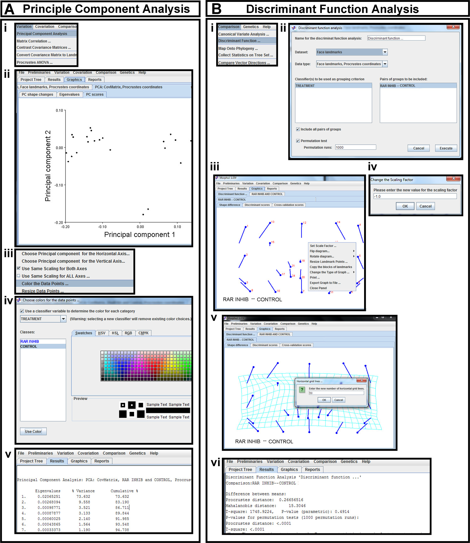
Figure 6. Statistical analysis in morphometric software. (A) Principal Component Analysis (PCA) (i) PCA is selected from the Variation tab. (ii) The first two principal components of Procrustes landmarks are displayed as a scatterplot in the PC scores tab. (iii) A pop-up menu is brought up in the plot space. This menu is used to change which principal components are plotted against each other (red arrow) and to color the data points (highlighted in blue). (iv) The data points are colored according to the classifier variables in the pop-up menu. (v) Percentage of variance captured by each principal component is viewed in the Results tab. (B) Discriminant Function Analysis (DFA) (i) DFA is selected from the Comparison tab. (ii) The data set of Procrustes coordinates is selected for DFA, and the previously uploaded classifiers are chosen for grouping. The desired groups to be compared are chosen and permutation tests are run. (iii) DFA results are displayed as a vector map in the Shape Difference tab. A pop-up menu in the plot space can be used to orient the image correctly. (iv) By selecting the Set Scale Factor tab in the pop-up menu, the sign of the scale factor can be changed. (v) The vector map is changed to a transformation grid with the desired number of grid lines by choosing Change the Type of Graph in the pop-up menu of the vector map. (vi) The Mahalanobis and Procrustes distances and corresponding p-values are viewed under the Results tab. Please click here to view a larger version of this figure.
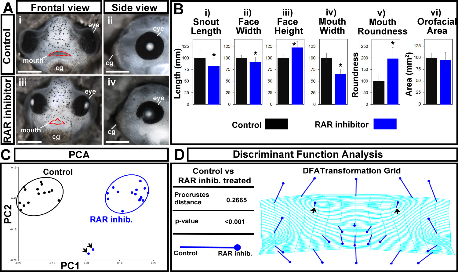
Figure 7. Orofacial analysis of control and RAR inhibited treated embryos. (A) (i,ii) Representative images of controls. Scale bars = 270 µm. (iii,iv) Embryos treated with a 1 μM concentration of the RAR inhibitor, BMS-453. Scale bars = 260 µm. (i,iii) Frontal views. Mouth opening is outlined in red dots. (ii,iv) Side views. cg: cement gland. (B) Traditional orofacial dimensions of control (black) and inhibitor treated (blue) embryos. (i) snout length, in mm (ii) face width, in mm (iii) face height, in mm (iv) mouth width, in mm (v) mouth roundness, a unit-less number determined in ImageJ using the equation: (4 × [Area]) / (π × [Major axis]2). (vi) Orofacial area, in mm2. Asterisks indicate significance as determined by Student’s T-test assuming unequal variance. α < 0.05. (C) Principal Component Analysis. Controls are in black and RAR inhibitor treated embryos are in blue. Black arrows indicate outliers. PC1 = 73.63%, PC2 = 9.56%. (D) Discriminant Function Analysis displaying the Procrustes distance and p-value, in addition to a transformation grid. Closed circle end of vector is landmark position in RAR inhibitor treated embryos. The end of the line of the vector is the landmark position in controls. Black arrows indicate shift in nasal landmarks. Please click here to view a larger version of this figure.
Xenopus laevis has become a useful tool for dissecting the developmental mechanisms underlying orofacial development; however, there are currently no protocols describing size and shape changes of this region in frogs. The method described here will contribute significantly to the field of orofacial development by allowing for more rigorous quantification of orofacial phenotypes in Xenopus and other vertebrates.
The first, most critical aspect of properly executing this protocol is the ability to measure facial dimensions and determine landmark placement both accurately and reproducibly. To this end, it is crucial that embryonic faces be photographed at the same angle, direction and magnification. Particular care must be taken to obtain precise measurements of the snout length, as it is difficult to manipulate embryos laterally and achieve consistent placement. Having a single person perform all measurements on the same day minimizes this type of error, while maximizing the reproducibility of the results. The second most critical aspect of ensuring good results is the reduction of unnecessary variability, such as developmental differences or genetic background. This is especially important when assessing statistical significance between subtle defects. Embryos, therefore, need to be at the same stage when treated and photographed. Moreover, care should be taken to ensure developmental rates are equivalent between and among treatment groups. To decrease such problems with variability, make sure that all embryos are from the same parents and are stage matched at the beginning of the experiment. Also reduce external sources of variability such as different buffer sources and volumes, different numbers of embryos, and distributions in the culture dishes (for example, prevent crowding).
A key step in assessment of shape changes through geometric morphometrics is the alignment of landmark coordinates via Procrustes fit. By application of this mathematical algorithm, any information about size or differences in rotation of the image is removed. The subsequently generated covariance matrix determines the unstandardized correlations of landmark coordinates among all the embryos in the data set, on which multivariate statistical techniques- such as principal component or discriminant function analyses- can be performed.
A principal component analysis (PCA) reduces a complex sample to a smaller set of variables called principal components26. The first component accounts for the most variance within the sample set, with each subsequent component accounting for the rest. By plotting the first two components against each other using morphometric software, samples that are most similar cluster together. In this way, PCA discriminates groups within a sample set, while simultaneously determining the variation within them. In some cases, groups may not be clearly distinguished from each other and overlap along either or both axes. In this case, it is advantageous to plot other components (for example, PC3) in order to reveal subtle features by which groups are discriminated. This is especially relevant when the total variance is more evenly distributed among the first several variables.
The discriminant function analysis (DFA) of Procrustes fit data determines whether samples in a data set are effectively discriminated into groups by the continuous variables that define them. Samples are therefore classified into groups prior to analysis, and the variables are translated into components called discriminate functions to determine the statistical relationship between the groups27. Prior to running this analysis, it is important to indicate the number of permutation tests. These permutation tests randomize the data such that any assumptions about its distribution are eliminated. More permutation test iterations increase the accuracy of the p-value. When visualized as a transformation grid, significant changes in landmark position between the groups being compared are displayed. Further, the warping pattern of the grid reveals where shape changes occur. The drawback of this analysis is that it can only be utilized for comparison of two groups. If there are three or more groups in a sample set for comparison, it is better to perform a canonical variate analysis. This is similar to a DFA in that it generates a statistical p-value; however, it shows changes occurring over the entire sample set in addition to those occurring between individual groups within that set.
The major limitation of this orofacial quantification protocol is that it can only be applied to two-dimensional data. Our future goals include using CT scanning or confocal microscopy to develop similar methods for analysis of three-dimensional data. On the other hand, working with two-dimensional images is also one of the major strengths of this protocol. Only basic stereoscopes fitted with cameras are needed for capturing images of the embryonic face. The Openware utilized for this data analysis also increases the accessibility of this method, while decreasing the cost. Further, an advanced knowledge of sophistical imaging, statistical analyses, or computer programming is not required to extract meaningful and significant results from the data. In fact, this technique is currently being taught as part of an undergraduate laboratory course in the VCU department of biology. Thus, the orofacial quantification protocol presented here is easy to learn and apply in a short period of time. As a video representation, critical steps such as positioning embryos and navigating the software are highlighted to ensure the protocol can be successfully utilized by even untrained students and researchers. In summary, this protocol will provide a valuable resource for the research community and as a teaching tool.
The authors have nothing to disclose.
Start-up monies to A. Dickinson from VCU supported this work.
The authors wish to acknowledge Dan Nacu for his artistic talent in creating the schematic illustration.
Name of the reagent | Company | Catalogue number | Comments (optional) |
Dissecting microscope | Zeiss | fitted with AxioCamICC1 camera | |
Dumont #5 Inox forceps | Fine Science Tools | 11251-10 | |
Sterile, disposable scalpel | Sklar | 06-2015 | |
24-well plate | Fisher Scientific | 087721 | |
Standard Disposable transfer pipettes | Fisher Scientific | 13-711-7M | |
150 mm X 15 mm Petri dishes | Falcon | 351058 | |
Incubators | Ectotherm | set to 15C or 20C | |
Modeling Clay | Premo, or other non-toxic modeling clay | in black or white | |
Straight teasing needle | Thermo Scientific | 19010 | |
Capillary Tubing (for needles) | FHC | 30-30-1 | Borosil 1.0mm OD x 0.5mm ID/Fiber, 100 mm each |
Needle Puller, Model P-97 | Sutter Instrument Co, | Needle Puller: P-97 Flaming/ Bown micropipette puller Filament: FB300B | For filaments, use Sutter 3.00mm square box filaments, 3.0mm wide. |
Pipettemen | Gilson | F144802, F123600, F123602 | |
BMS-453 | Tocris | 3409 | |
DMSO | American Bioanalytical | AB00435-01000 | |
Cysteine | Sigma-Aldrich | 52-90-4 | |
Paraformaldehyde powder | Sigma-Aldrich | 158127 | |
Petri dishes | Falcom | 353003, 351058 | 100 mm diameter and 150 mm in diameter |
100% Ethanol | VWR | 89125-170 |