

Summary
Spatial distribution and temporal dynamics of plasma membrane proteins and lipids is a hot topic in biology. Here this issue is addressed by a spatio-temporal image fluctuation analysis that provides conceptually the same physical quantities of single particle tracking, but it uses small molecular labels and standard microscopy setups.
Abstract
It has become increasingly evident that the spatial distribution and the motion of membrane components like lipids and proteins are key factors in the regulation of many cellular functions. However, due to the fast dynamics and the tiny structures involved, a very high spatio-temporal resolution is required to catch the real behavior of molecules. Here we present the experimental protocol for studying the dynamics of fluorescently-labeled plasma-membrane proteins and lipids in live cells with high spatiotemporal resolution. Notably, this approach doesn’t need to track each molecule, but it calculates population behavior using all molecules in a given region of the membrane. The starting point is a fast imaging of a given region on the membrane. Afterwards, a complete spatio-temporal autocorrelation function is calculated correlating acquired images at increasing time delays, for example each 2, 3, n repetitions. It is possible to demonstrate that the width of the peak of the spatial autocorrelation function increases at increasing time delay as a function of particle movement due to diffusion. Therefore, fitting of the series of autocorrelation functions enables to extract the actual protein mean square displacement from imaging (iMSD), here presented in the form of apparent diffusivity vs average displacement. This yields a quantitative view of the average dynamics of single molecules with nanometer accuracy. By using a GFP-tagged variant of the Transferrin Receptor (TfR) and an ATTO488 labeled 1-palmitoyl-2-hydroxy-sn-glycero-3-phosphoethanolamine (PPE) it is possible to observe the spatiotemporal regulation of protein and lipid diffusion on µm-sized membrane regions in the micro-to-milli-second time range.
Introduction
Starting from the original “fluid mosaic” model by Singer and Nicolson, the picture of cellular plasma membrane has been continuously updated during the last decades in order to include the emerging role of cytoskeleton and lipid domains1,2.
The first observations were obtained by fluorescent recovery after photobleaching (FRAP) unveiling that a significant fraction of membrane proteins is immobile3-5. These pioneering studies, although very informative, suffered from the relatively poor resolution in space (microns) and time (seconds) of FRAP setups. Also, being an ensemble averaging measurement, FRAP lacks in giving information on single molecule behavior.
In this context, the possibility to specifically label a single molecule with very bright tags (allowing the study of the diffusion process one molecule at a time) has been very successful. Particularly, by pushing the time resolution of the Single Particle Tracking (SPT) approach to the microseconds timescale, Kusumi, et al. gained access to unknown features of lipid and protein dynamics that greatly contributed to the recognition of the role of actin-based membrane skeleton in membrane physiology6,7. These findings generated the so-called the ‘picket and fence’ model, in which lipid and protein diffusion is regulated by actin-based skeleton. However, in order to have access to the huge amount of information provided by SPT many experimental issues have to be addressed. Particularly, the labeling procedure is typically composed by many steps like production, purification and introduction of the labeled species into the system. Furthermore, big labels, like quantum dots or metal nanoparticles, are often required to reach the sub-millisecond timescale and the crosslinking of the target molecules by the label could not be avoided in many cases. Finally, many trajectories have to be recorded to fit statistical criteria and concomitantly a low-density of the label is required to allow tracking.
Compared to SPT, fluorescence correlation spectroscopy (FCS), overcoming many of these drawbacks, represents a very promising approach to study molecular dynamics. In fact, FCS works well also with dim and dense labels, enabling to study the dynamics of fluorescent protein-tagged molecules in transiently transfected cells. Also, it allows reaching high statistics in a limited amount of time. Finally, despite the “high” density of labels FCS provides single molecules information. Thanks to all these properties, FCS represents a very straightforward approach and has been extensively applied to study lipid and protein dynamics both in model membranes and in live-cells8-10. Many different approaches have been proposed to increase the ability of FCS to reveal the details of molecular diffusion. For instance, it was shown that by performing FCS on differently-sized observation areas one can define an “FCS diffusion law” enlightening hidden features of molecular motion11,12. Besides being varied in size, the focal area was also duplicated13, moved in space along lines14-20 or conjugated with fast cameras21,22. Using these ‘spatio-temporal’ correlation approaches, relevant biological parameters of several membrane components were quantitatively described on both model membranes and actual biological ones, thus yielding insight into membrane spatial organization.
However, in all the FRAP and FCS applications described so far the size of the focal area represents a limit in spatial resolution that cannot be overcome. Several super-resolution imaging methods have been recently developed to bypass this limit. Some are based on localization precision, such as stochastic optical reconstruction microscopy (STORM)23,24, photoactivation localization microscopy (PALM)25, fluorescence PALM (FPALM)26, and single-particle tracking PALM (sptPALM)27: the relatively large amount of photons required at each snapshot, however, limits the time resolution of these methods to at least several milliseconds, thus hampering their applicability in vivo.
In contrast, a promising alternative for super resolution imaging have been opened by spatially modulating the fluorescence emission with stimulated emission depletion methods (STED or reversible saturable optical fluorescence transitions (RESOLFT))28,29. These approaches combine the shaping of the observation volume well below the diffraction limit with the possibility to use fast scanning microscopes and detection systems. In combination with fluorescence fluctuation analysis, STED microscopy allowed to directly probe the nanoscale spatiotemporal dynamics of lipids and proteins in live cell membranes30,31.
The same physical quantities of STED-based microscopy can be obtained by a modified spatio-temporal image correlation spectroscopy (STICS32,33) method that is suitable for the study of the dynamics of fluorescently-tagged membrane proteins and/or lipids in live cells and by a commercial microscope. The experimental protocol presented here is composed by few steps. The first one requires a fast imaging of the region of interest on the membrane. Then, the resulting stack of images is used to calculate the average spatial-temporal correlation functions. By fitting the series of correlation functions, the molecular ‘diffusion law’ can be obtained directly from imaging in the form of an apparent diffusivity (Dapp)-vs-average displacement plot. This plot critically depends on the environment explored by the molecules and allows recognizing directly the actual diffusion modes of the lipid/protein of interest.
In more details, as previously shown34, the spatio-temporal auto-correlation function of the acquired image series critically depends on the dynamics of the molecules moving in the collected image series (please note that the same reasoning can be applied in a line acquisition where just one dimension in space is considered). In particular, we define the correlation function as:
 (1)
(1)
where  represents the measured fluorescence intensity in the position x, y and at time t,
 ![]() and
and ![]() represents the distance in the x and y directions respectively,
represents the distance in the x and y directions respectively,![]() represents the time lag, and
represents the time lag, and ![]() represents the average. This function can be expressed as:
represents the average. This function can be expressed as:
 (2)
(2)
where ‘N’ represents the average number of molecules in the observation area, ![]() represents the convolution operation in space, and
represents the convolution operation in space, and  represents the autocorrelation of the instrumental waist. This latter can be interpreted as a measure of how the photons of a single emitter are spread out in space due to the optical/recording setup (the so called Point Spread Function, PSF, generally well approximated by a Gaussian function). Finally,
  represents the probability to find a particle at a distance
 ![]() and
and ![]() after a time delay
after a time delay ![]() . If we consider a diffusive dynamics, in which particles move randomly in all directions and net fluxes are not present, this function is also well approximated by a Gaussian function where the variance can be identified as the Mean Square Displacement (MSD) of the moving particle. Thus, the waist of the correlation function (also referred as
. If we consider a diffusive dynamics, in which particles move randomly in all directions and net fluxes are not present, this function is also well approximated by a Gaussian function where the variance can be identified as the Mean Square Displacement (MSD) of the moving particle. Thus, the waist of the correlation function (also referred as ![]() ), can be defined as the sum of the particle MSDs and the instrumental waist and can be measured by a Gaussian fitting of the correlation function for each time delay. The measured iMSD can be used to calculate an apparent diffusivity of the moving molecules
), can be defined as the sum of the particle MSDs and the instrumental waist and can be measured by a Gaussian fitting of the correlation function for each time delay. The measured iMSD can be used to calculate an apparent diffusivity of the moving molecules ![]() and an average displacement
and an average displacement![]() as:
as:
 (3)
(3)
 (4)
(4)
Few considerations on the experimental setup used can guide the reader throughout the following sections. In order to selectively excite the fluorophores on the basal membrane of living cells we will use a total internal reflection (TIR) illumination, using a commercial TIR fluorescence (TIRF) microscope (details can be found in the material section). Moreover, in order to collect the fluorescence we will use a high magnification objective (100X NA 1.47, high numerical aperture is required for TIRF illumination) and an EMCCD camera (physical size of the pixel on the chip 16 μm). To reach a pixel size of 100 nm we apply an additional magnification lens of 1.6X. As discussed below, a time resolution below 1 msec would be required to properly describe the dynamics of fast membrane lipids below 100 nm. In order to reach this temporal resolution we need to select a region of interest (ROI) smaller than the whole chip of the camera (512 x 512). In this way, the camera will read a reduced number of lines increasing the time resolution. However, in this readout regime the frame time would be limited by the time required to shift the charges from the exposure to the readout chip on the camera and is usually in the order of milliseconds for 512 x 512 pixel EMCCD. To beat this limit, an emerging technology allows shifting the ROI-lines only instead of the whole frame, with a practical effective reduction of the exposed chip size (called Cropped Sensor Mode in our EMCCD). For this configuration to be effective, the chip outside of the ROI must be covered by a couple of slits mounted in the optical path. Thanks to this setup a time resolution down to 10-4 seconds can be achieved. Please note, however, that this approach can be coupled with many different experimental setups, as explained in the ‘discussion’ section.
Demonstration of the method will be provided in live cells, by using both an ATTO488 labeled 1-palmitoyl-2-hydroxy-sn-glycero-3-phosphoethanolamine (ATTO488-PPE) and a GFP-labeled variant of the Transferrin Receptor (GFP-TfR). In the case of ATTO488-PPE this approach can successfully recover an almost constant Dapp as a function of average displacement indicating a mostly free diffusion, as previously reported30,35. By contrast, TfR-GFP shows a decreasing Dapp as a function of average displacement, suggesting partially-confined diffusion6. Moreover, in the latter case it is possible to quantify the local diffusion constant and the average confinement area over many microns on the membrane plane.
Subscription Required. Please recommend JoVE to your librarian.
Protocol
1. System Calibration
- Point Spread Function (PSF) calibration
- Dilute 10 µl of 30 nm fluorescent bead solution (about 5 μM) in 90 µl of distilled water and then sonicate the solution for 20 min. Cut a square (1 cm x 1 cm) piece of agarose gel (3%) and deposit 10 µl of the solution on the top of the gel. Overturn the piece of gel on the bottom glass of a 2 cm Petri dish and squeeze the drop on the glass.
- Turn on the acquisition setup, put the sample in the holder, set the camera exposure and EMgain (100 msec and 1,000 are good parameters but optimize according to the system) and wait for the camera to cool down.
- Set camera exposure to 100 msec, camera EMgain to 1,000, acquisition mode to Frame Transfer, 100 repetition and auto save setting.
- Using the eyepiece and transmitted light focus on the border of the gel and then move the objective to the center of the gel, adjust the focus and start the laser alignment procedure (in LAS AF, select ‘TIRF setup’ and follow the auto alignment procedure).
- Find a field of view with isolated single spots, accurately focus on the brighter spot (that usually represents beads aggregate) as a reference, acquire 100 frames and repeat the step 5-6 times in order to acquire several single spots.
- Import the acquired series to a data processing program and average the stack in time (Figure 1A) and select a single isolated bead. Take care to select the smallest ones to avoid particle aggregates.
- Fit the selected intensity distribution (an example of single beads profile is presented in Figure 1B) with a Gaussian function using the command “gaussfit” (in the ICS-Matlab tools in the Materials in Matlab). Verify the goodness of the fit by inspecting the obtained residuals (an example of fitted Gaussian profile with the corresponding residuals is presented in Figure 1B).
- Camera calibration
- Turn on camera and wait for the camera to cool down. Set camera acquisition setting, (i.e., for the used camera we set the exposure to 0.5 msec, camera EMgain to 1,000, acquisition mode to Cropped Mode, the ROI size to 32 x 128, 10,000 repetitions) and start the acquisition of the camera background signal.
- Import acquired frame series to a data processing program. Calculate and inspect the average intensity in each pixel in order to verify that the camera background is approximately flat in the selected region of the chip. In Cropped Mode, remove the first and the last few horizontal lines (3 to 10 depending on the size of the ROI) for each frame because the camera background is usually biased in the border lines.
- Create a histogram of the values (also defined Digital Level, DL) in acquired images stack (using command ‘hist’ in Matlab) and plot the logarithm of resulting frequency (using semilogy command in Matlab). An example of DL distribution for camera background is presented in Figure 2.
NOTE: If the camera is working well, the plot will show an approximately Gaussian peak (a parabolic profile in log-scale) representing the distribution of values associated to zero photon followed by an exponential decay (a line with negative slope in log-scale) that represents the distribution of values associated to 1 photon (Figure 2). In particular, the center and the variance of the Gaussian function represent the camera offset and error, respectively, while the decay constant of the exponential part represents an estimation of the DL assigned by the camera to each single photon. In Matlab use the section “CalibrateCamera” of the Script in supporting materials. - Repeat the operation for all the selected Camera EMGain and Gain.
2. Labeled Cell Preparation
- To prepare the liposomes required for lipid incorporation 36, dissolve separately 1 mg of DOPE (1,2-dioleoyl-sn-glycero-3-phosphoethanolamine), 1 mg of DOTAP (1,2-dioleoyl-3-trimethylammonium-propane), and 1 mg of PPE-ATTO488 in 1 ml of chloroform. Mix together 0.5 ml of DOPE solution, 0.5 ml of DOTAP solution, and 25 µl of PPE-ATTO488 solution and dry under vacuum for 24 hr. Add 0.5 ml of HEPES buffer 20 mM, vortex for 15 min and sonicate for 15 min at 40 °C.
- To prepare the cell, wash 3 times with PBS a p100 dish of confluent CHO-K1 (Chinese Hamster Ovary), add 1 ml of trypsin and store in incubator for 5 min. Suspend detached cells adding 9 ml of DMEM/F12 medium supplemented with 10% of FBS and seed 150 µl of cell solution in a Petri dish containing 800 µl of the same medium.
- Store in incubator for 24 hr at 37 °C and 5% CO2. For lipid incorporation, replace cell medium with 500 µl of serum-free medium; after 30 min, add 2 µl of liposomes solution; after 15 min wash with PSB and add new DMEM/F12 medium for imaging.
- For Transfection, transfect cells according to Lipofectamine protocol (Manufacturer instructions) using TfR-GFP plasmid and store 24 hr in incubator before imaging.
3. Data Acquisition
- Setup preparation
- In order to thermostat the microscope, 24 hr before the experiment turn on the incubator.
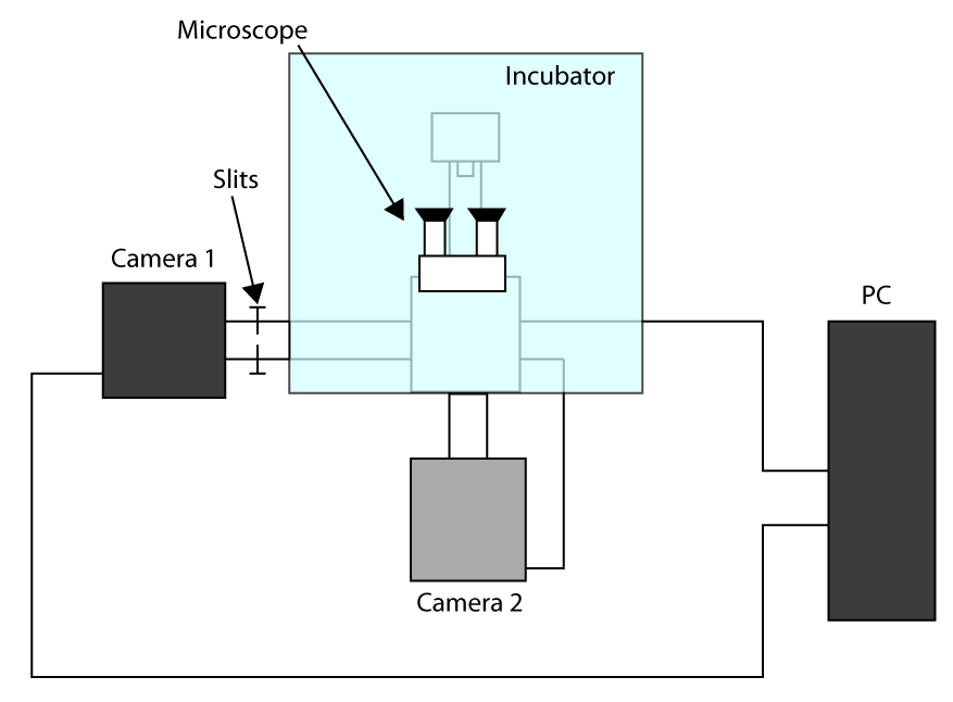
- In order to apply the fastest achievable acquisition time, work in Cropped Sensor Mode (see introduction) and use a first camera for imaging (camera 1) and second camera to select the cell (camera 2). A scheme of the setup configuration is presented in Supplementary Figure S1. Then, to align the two cameras turn on the microscope and wait for the cameras to cool down.
- Set on both cameras the parameters for transmitted light imaging (i.e., 20 msec for exposure time, 1 for EM Gain) and put the microscope in Bright Field mode.
- Put the samples in the holder and focus using eyepiece, send the light to camera 1 and gently push the slits allowing light only on the ROI used for cell imaging (here a 32 x 32 pixels ROI).
- Move a cell in the selected region and send the light to the camera 2, then draw a ROI in the software that control camera 2 in order to have a reference.
- Imaging (Figure 3A)
- First of all, align the TIRF laser according to the procedure of your setup. In our setup, select the ‘TIRF setup’ and start the auto alignment procedure. When the laser is aligned set 70 nm of penetration depth (about 70°).
- Set exposure time to 70 msec and EMGain to 100 on both camera 1 and camera 2; then, select a cell using camera 1, then send the light on camera 2 and accurately focus the cell membrane. Set the minimum exposure on camera 2, 1,000 EMGain, Cropped Sensor Mode, 105 repetitions and set autosave as fits files (Flexible Image Transport System, a format that can be easily managed).
- Start the acquisition to record the image series. Release the Gain and the cropped Mode to allow temperature stabilization before acquiring a new cell, then repeat the last two steps in order to acquire 8-10 cells.
4. Calculation of the Mean Square Displacement from Imaging (iMSD)
NOTE: The following protocol can be directly applied to raw data. At the same time, the whole protocol is valid for data acquisitions simulated both in Matlab and in SimFCS. The link to the corresponding tutorials can be found in the ‘Materials’ section.
- Calculation by Matlab
- Import the acquired series to Matlab using ImportImageSeries script. Calculate the average intensity of each image in time using the command mean on the first 2 dimensions and use plot to see the resulting vector.
- If more than 10% of photobleaching is present, discard the series or remove the first part of them. If it is lower, try to correct the effect on the correlation function by subtracting to each image its average intensity, as shown before37.
- Calculate the average intensity of each pixel by using mean on the third dimension and see resulting image.
NOTE: Particular attention is required in order to avoid artifactual correlations. In fact, as previously shown for similar techniques38, cell borders as well as out of focus vesicles could introduce a strong correlation. If the inspection of the average image reveals cell borders or out of focus vesicles, try to exclude the region involved otherwise discard the acquisition. To correct the effect of this immobile structures subtract the average temporal intensity from each pixel39. - Calculate the spatiotemporal correlation (G(ξ,χ,τ)) by using the function CalculateSTICScorrfunc. Remove G(ξ,χ,0) because the correlation due to the shot noise in low-light regime dominates G(0,0,0); the correlation due to the detector dominates the G(±1,0,0), and particle movement during the exposure time could deform G(ξ,χ,τ) for τ=0 by increasing the measured waist (this effect disappears for τ>0)34.
- Average G(ξ,χ,τ>0) using a logarithmic time-bin to reduce the noise by using “LogBinStack” function in Supporting Material and then fit the resulting G(ξ,χ,τ) using the function “gaussfit” of the ICS-Matlab tools in the Materials to recover the iMSD (the second column of the resulting array).
- Plot the obtained waist σ(τ)2 (iMSD) as a function of time. If the data are too noisy, try to increase the number of acquired frames, increase the laser power, average more G(ξ,χ,τ) together.
- Calculation by SimFCS
- Open the acquired files with ImageJ using BioFormat importer plugin and save acquired series as Tiff sequence.
- Open SimFCS and select RICS tool and select File>Import Multiple Images (Supplementary Figure S2).
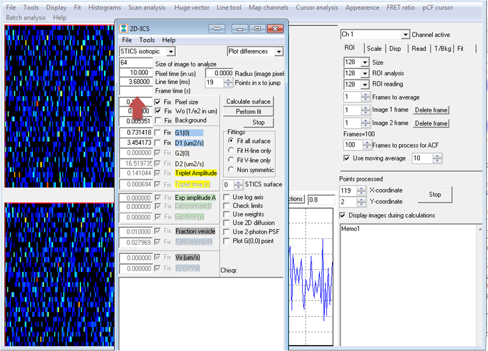
- Select Fit, insert the correct acquisition parameters and close the fit window (Supplementary Figure S3).
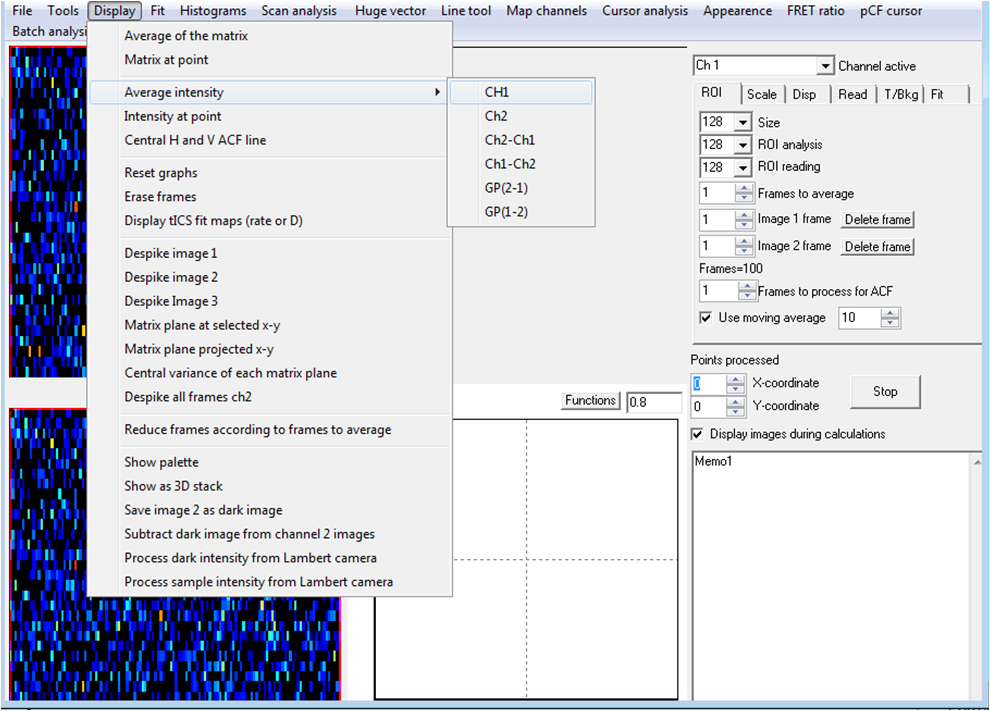
- Select Display>Average Intensity>CH1 and verify the presence of photobleaching (Supplementary Figure S4).
- If more than 10% of photobleaching is present discard the series or if it is possible load again the image sequence removing the first part of the series.
- If bleaching it is lower than 10% select Tools>iMSD>Set Parameters, check ‘Use moving average’, set in the ROI panel on the left a number of frame for the moving average paying attention that the correspondent time is higher than the characteristic diffusion time (for particle moving at 1 µm2sec-1 a time of 10 sec is a good moving average)
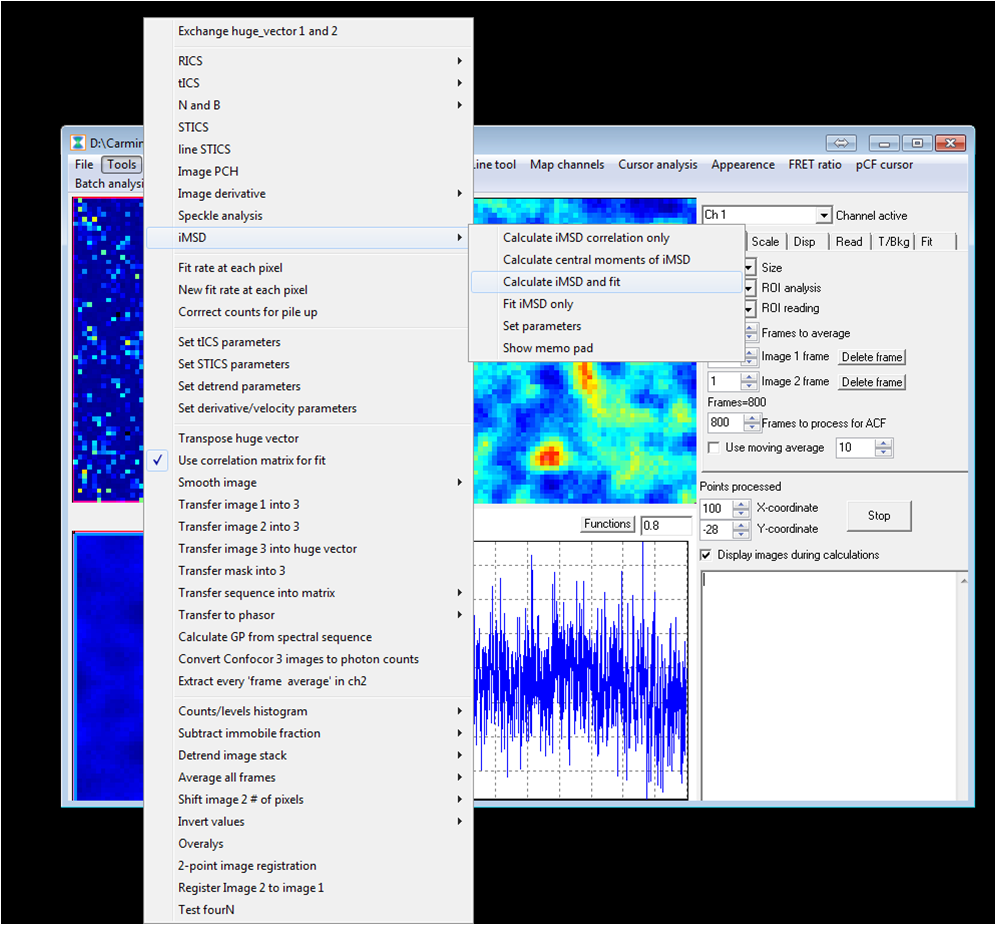
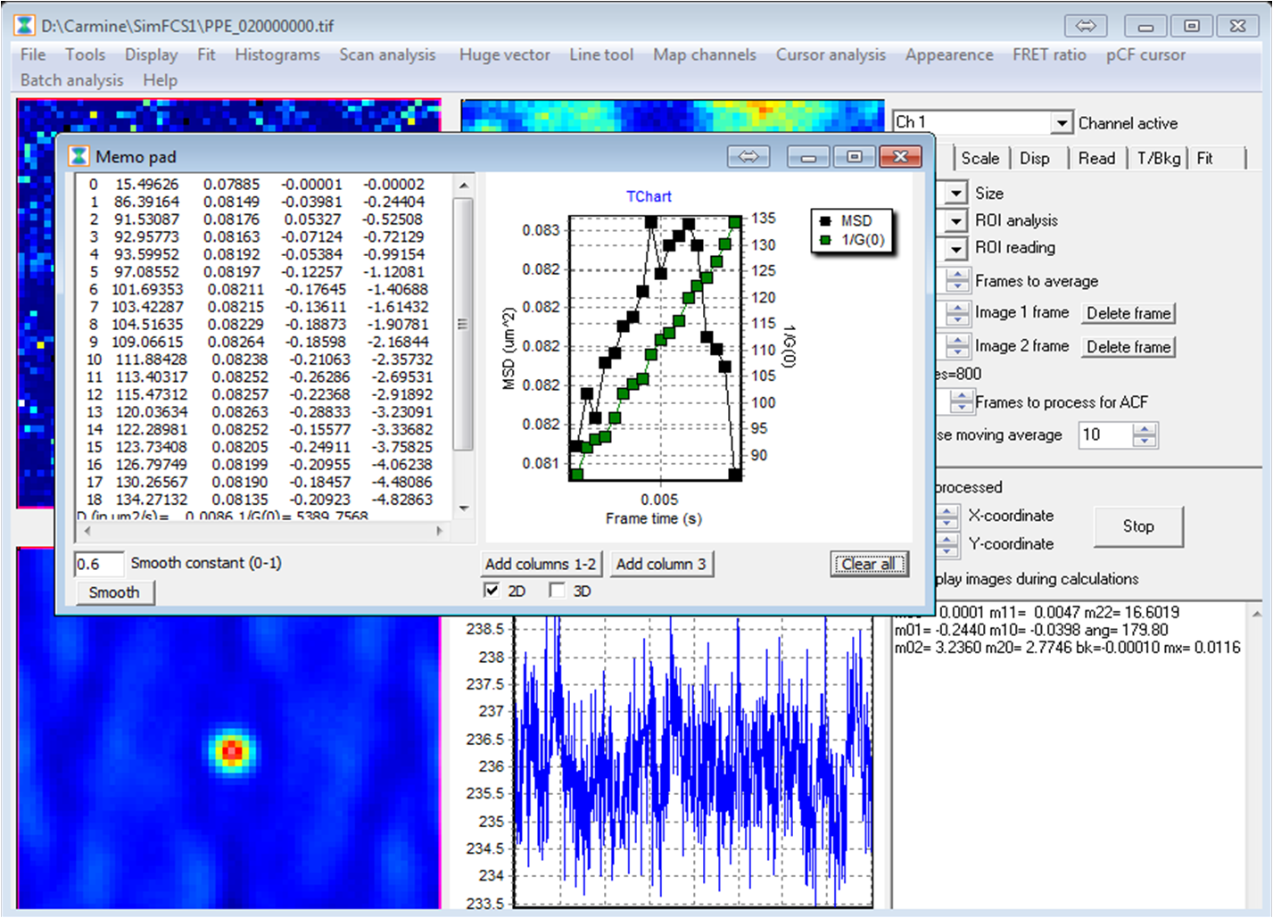
- Select Tools>iMSD>Calculate iMSD (Supplementary Figure S5) and fit and export the iMSD from the memo pad (Supplementary Figure S6).
5. Calculation of the Diffusion Law from the iMSD
- Fit the first few points to extrapolate the intercept (σ02) (5 points are usually enough but more points can be fitted if they show a linear behavior) and compare this value with the previously measured PSF2. If they are comparable, the dynamics of isolated fluorophores are being followed. By contrast, if σ02 >> PSF2 try to acquire faster to ensure that no hidden dynamics are present34.
- Calculate the apparent diffusivity (Dapp) and the average displacement (R) using equations 3 and 4 (see Introduction).
- Plot Dapp as a function of R to obtain a diffusion law comparable with what is measured with spot variation based FCS12 (Figure 3D).
Subscription Required. Please recommend JoVE to your librarian.
Representative Results
In order to calibrate the instrumental waist, the image of a single fluorescent nano-bead can be measure as described in Protocol step 1.1. A typical fluorescent image of these beads is presented in Figure 1. The fitting of intensity distribution by a 2D Gaussian function gives back good residuals and allows measuring the instrumental waist at 270 nm. This value is in good agreement with the expected diffraction limit estimated by the Rayleigh equation. This calibration is not necessary for the measurement of particle dynamics but it is required to measure the apparent particle size.
A typical frequency distribution of camera background is presented in Figure 2. The peak at about 180 DL is due to the camera response to no photon, and it represents the contribution of Analog Digital (AD) converter. This contribution can be approximated as a Gaussian distribution to estimate the offset and the variance introduced by the signal recording. Above 200 DL the digital level distribution becomes exponential (linear in logarithmic scale) and represents the average camera response to a single photon. Fitting this part with an exponential distribution allows the measurements of the average DL assigned to each single photon. The higher is the ratio between the average DL assigned to each photon and the AD converter error, the lower will be the noise in the calculated correlation function. Moreover, the average single photon response allows the estimation of the camera dynamic range.
A diagram of the complete experimental procedure is summarized in Figure 3 and a picture of Atto488-PPE insertion into the membrane is represented in Figure 4A. A representative TIRF image of the basal membrane of a CHO cells labeled with Atto488-PPE is presented in Figure 4B. Several bright spots may be present outside the cell due to liposomes stacked on the glass. They can be discarded by selecting a ROI on a membrane portion mostly uniform in fluorescence (i.e., the cellular plasma membrane). As expected the measured diffusion law (Figure 4C) for this lipid is flat, indicating a mostly free diffusion as previously shown by STED-FCS measurements30,35. It is worth mentioning that all the shown displacement values are below the diffraction limit, clearly indicating the ability of this approach to super-resolve average molecular displacements well below the diffraction limit and down to few tens of nanometers.
A schematization of TfR-GFP dimer insertion into the membrane is represented in Figure 5A. Many studies showed that the cytoplasmic tail of this receptor interacts with the membrane skeleton, which in turn acts as a fence for the receptor mobility12,40. A representative TIRF image of a CHO cell expressing TfR-GFP is presented in Figure 5B. Low fluorescence intensity cells should be preferred, as the membrane is closer to the native condition and the probability of artifacts related to the over-expression is minimized. In addition, the central part of the cell should be avoided, as the effects of out-of-focus fluorescence (from cytoplasm, for instance) may be present. As expected the measured diffusion law (Figure 5C) for TfR-GFP shows a first flat behavior below 100 nm, with an average Dapp of about 0.7 µm2sec-1, followed by consequent rapid decrease in apparent diffusivity down to 0.2 µm2sec-1 (the value typically measured by diffraction-limited FCS12). This result shows that our approach can easily measure the average displacement of GFP labeled proteins with a resolution of few tens of nanometers. Moreover the spatial scale at which Dapp starts to decrease sets the characteristic spatial scale of protein partial confinement by the membrane skeleton at around 120 nm, in keeping with previous estimates6.

Figure 1. Calibration of Point Spread Function. (A) Pseudocolor image of an isolated bead and beads aggregates. (B) 3D plot of the intensity profile of an isolated bead shows a well-defined Gaussian profile. (C) Fit of the intensity distribution by a Gaussian function (upper panel) with the corresponding residuals (lower panel). The good agreement between the fitted distribution and the measured intensity profile is also a proof that the instrumental PSF can be approximated by a Gaussian function. Please click here to view a larger version of this figure.

Figure 2. Calibration of Camera response to single photons. The figure shows the Digital Level (DL) distribution for camera background in a 32 x 128 ROI, exposure 0.5 msec, in Cropped Sensor Mode. The peak at about 180 DL represents the camera response to no photons. Particularly, it represents the contribution of the Analog Digital (AD) converter and can be approximated by a Gaussian function to estimate the offset and the variance introduced by the signal recording. Above 200 DL the distribution of digital levels becomes exponential and represents the average camera response to a single photon. The measurement of these parameters allows estimating the density of photons that are recorded during the acquisition. Please click here to view a larger version of this figure.

Figure 3. Schematization of the method. (A) Wide field imaging by EMCCD camera is applied to reach sub-millisecond resolution, while TIRF microcopy is exploited to provide accurate optical sectioning of the plasma membrane. (B) The resulting stack of images is autocorrelated in order to calculate the average spatial-temporal correlation function. This correlation function is well approximated by a Gaussian function (see Introduction) and it spreads out in time according to particle displacements. (C) Thus, in order to quantify the spreading of the correlation function due to molecular displacement, fitting with a Gaussian function is performed. This allows measuring the molecular ‘diffusion law’ directly from imaging, in the form of apparent diffusivity vs average displacement plot. (D) Thanks to this plot, molecular diffusion modes can be directly identified with no need for an interpretative model or assumptions about the spatial organization of the membrane. In fact, freely diffusing molecules will display a constant apparent diffusivity as their mobility does not depend on the spatial scale of the measurement. By contrast, partially confined molecules will display a quite constant apparent diffusivity for displacements smaller than confinement size, then a decreasing diffusivity for spatial scales bigger than confinement size. Thus, the appearance of a reduction in the apparent diffusivity can be interpreted as a fingerprint of transient confinement, while the related spatial scale can be used to estimate the spatial extension of the confinement. Please click here to view a larger version of this figure.

Figure 4. ATTO488-PPE diffusion law in live cell membranes. (A) Schematic representation of ATTO488-PPE insertion in cell membrane. (B) TIRF image of CHO basal membrane labeled with ATTO488-PPE: a ROI (red box) is selected in a mostly uniform part of the cell, avoiding cell border and highly fluorescent spots. (C) The diffusion law measured in the selected ROI shows a flat behavior confirming a free diffusion model for this component. Please click here to view a larger version of this figure.

Figure 5. TfR-GFP diffusion law in live cell membranes. (A) Schematic representation of TfR-GFP insertion in cell membrane: the cytoplasmic tail of the receptor interacts with the membrane skeleton, that acts as a fence for receptor mobility. (B) TIRF image of CHO expressing TfR-GFP: a ROI is selected preferring low expressing cells to avoid artefacts due to overexpression. (C) The diffusion law of TfR (black dots), unlike PPE (gray line, taken from Figure 4), shows the typical behavior of partially confined diffusion where a first flat part is followed by a decrease in Dapp. Please click here to view a larger version of this figure.
Subscription Required. Please recommend JoVE to your librarian.
Discussion
Single particle tracking (SPT) represents one of the most common strategies to study molecular dynamics and it has the great advantage of measuring particle trajectories. This in turn allows probing the behavior of even few labeled particles in a complex system. However, to reach this advantage SPT typically needs a low density of the probe and very bright labels. Particularly, to gain high temporal resolution (μsec range) inorganic probe are usually required (e.g., quantum dots or metal nanoparticles): in this case a complex procedure of production, labeling and insertion into the system is necessary. Compared to SPT the present method shows some key advantages. First of all, this approach can be used in conjugation with fluorescent proteins. Thus, compared to SPT, a higher temporal resolution is achieved (on the same label) thanks to the lower amount of photons required34. More in detail, this property allows pushing the temporal resolution below 10−3 sec also when using encodable fluorescent proteins, and this timescale gives exclusive access to the nanoscale dynamics of membrane constituents. Finally, it is worth noting that molecular diffusion laws are described by analyzing the full space-time correlation function, with no need to track each molecule.
The comparison with STED-based FCS is also interesting. In a STED-FCS measurement the average transit time of molecules for decreasing observation volumes is measured by the temporal correlation of the fluorescence signal. This allows obtaining a local measurement of the molecular dynamics also below the diffraction limit. In the presented approach the diffusion law is measured as the average of all the particles moving in the selected ROI, observed by means of standard, diffraction-limited, observation volume. However, reported results demonstrate that this method is not limited by diffraction, but only by the temporal resolution available. In fact, although a diffraction-limited acquisition is used to detect fluctuations (analogously to what is done in other super-resolution techniques, such as PALM and STORM), molecular displacements well below the diffraction limit can be (directly) calculated, as already demonstrated by using STICS to measure molecular flows32. Moreover, unlike STED-FCS, this approach can be easily applied to a wide range of commercial and existing microscopy setups, such as raster scanning microscopes or wide field camera-based microscopes. It is worthy of mention that STED-FCS measurements of molecular diffusion laws strictly require a fluorophore-dependent calibration of the size of the instrumental waist. Oppositely, the measurement presented here does not require a system calibration (needed only for the estimation of particle size).
The actual resolution in the measurement of particle displacements by the presented method depends on how accurately we can measure the correlation function. Consequently, it is not inherently limited by diffraction, analogously to the SPT case where the resolution depends on how accurately the particle “image” is measured. To measure a significant correlation in less than 1 min for the proposed experiments, few photons (usually below 10 photons) for each particle in each frame are enough. In fact, the contribution of all the observed particles is averaged together when the correlation function is calculated, even if particles are not isolated. This property is intrinsic of fluctuation correlation methods and allows using dim and dense labels, such as fluorescent proteins transfected in live cells.
With this in mind it appears clear that the minimum measurable displacement depends on the diffusivity of the particle and on the time resolution of the imaging setup. As an example, please consider diffusion of molecules on the cell membrane, where the maximum measured diffusivity for proteins or lipids is around 5 μm2sec-1. Under these conditions, we need a time resolution of approximately 10-4 sec to catch an average displacement of 50 nm. This time resolution can be achieved by fast scanning microscopes along single lines or by fast EMCCD camera, where time resolution coincides to the exposure time, as showed here.
An additional essential requirement for this method to accurately describe molecular dynamics is a correct spatial sampling. In fact, in order to fit the correlation function we need a spatial sampling (pixel size) lower than the waist of the instrumental PSF. In most commercial microscopes (confocal or wide field), the PSF waist spans from 200 nm to 500 nm (depending mainly on the numerical aperture of the selected objective and on the wavelength used) and can be easily measured by a calibration experiment using nano-sized fluorescent beads. Thus, a pixel size of 70-150 nm (3 times lower than the instrumental waist) can be enough. However, the pixel size can be adapted to the system under study taking into account a simple rule: lower the pixel size, higher the accuracy in the description of the correlation function. Furthermore, the minimum size of the image to be acquired has to be at least 3-times larger than the maximum displacement of interest (plus the instrumental waist). This is required in order to reach a good convergence of the fitting algorithm and a statistically significant sampling of molecular displacements. As an example, to study average molecular displacements smaller than few hundreds of nanometers (e.g., 200 nm) an image size of few microns is enough. Moreover, the total number of pixels (taking constant the pixel size) impacts on the quality of the correlation function. In fact, a larger image allows averaging more information in the correlation function, even if at expense of the time resolution. Concerning the camera-based system used here, please note that the physical size of the pixel on the chip is fixed. Consequently, decreasing the pixel size lowers the signal in each pixel (that depends on the square of the pixel size), decreases the field of view, and requires higher magnification power. On the other hand, in a scanning system, where the observation area is fixed, decreasing the pixel size usually results in an increased pixel number at the expense of the time resolution.
Few details about the detector used have to be discussed. Unlike single-photon detectors, EMCCD systems measure an average intensity (digital level, DL) that is not directly proportional to the collected light due to the presence of an offset. Even if this offset is low compared to the dynamic range of the camera (few hundred compared to 216 in 16 bit readout) and negligible in experiments where many photons are collected, it has to be taken into account to obtain a correct normalization of the correlation function. Also, the offset can be used as a reference in low-light conditions in order to identify the amount of signal collected. Moreover, in order to estimate the average amount of photons that are collected during the acquisition, the average digital level associated to each collected photon has to be measured. This quantity can be retrieved by exposing the camera to a very low light intensity (e.g., the background light in the room); in fact, in this case, we can reasonably assume that just single photons reach the camera, i.e. the measured intensity can be related to zero or one photon only.
Finally, let us comment on how some alternative acquisition systems (i.e., different microscopy setups) can be used to perform the presented measurements. First of all, the ‘W’factor in Equation 2 (that represents the autocorrelation of the instrumental PSF) can be adapted to the particular acquisition system used in order to fit the experimental correlation function. As previously shown34, an easy case is the acquisition whit a laser scanning microscope when the scanning speed is significantly higher than particle dynamics. In such a case, in fact, the movement of particles during the acquisition time (i.e., line time) can be considered negligible and the correlation function is well approximated by a Gaussian function. In the context of the emerging imaging technologies, an interesting approach is based on the possibility to produce very thin light sheets (1-2 μm) through the sample41. The light sheet allows selective illumination of a single plane (Single plane illumination microscopy, SPIM) in the sample and, combined with a camera-based acquisition system, fast optical sectioning in 3D42. Because of these characteristics, SPIM has been successfully conjugated with FCS43 and could represent a valid tool to extend the presented analysis to 3D environments, such as the cytoplasm or the nucleus of living cells.
Summarizing, from an experimental point of view this approach requires only the access to a microscope equipped with a fast acquisition module. The protein of interest can be tagged with any fluorescent protein or organic fluorophore, thus allowing also for multicolor imaging. In this context, we envision the possibility to use cross-iMSD analysis to select sub-populations of molecules and reveal interactions and co-diffusion on live cell membranes. Finally, we believe that this approach may represent a powerful tool to study proteins and/or lipids undergoing dynamic partitioning within nanodomains on the plasma membrane. In this case, the highly-variable size and lifetime of the nanodomains introduce an additional level of complexity in real data which would require further methodological implementations including 2-color imaging, local analysis (e.g., 2D pair correlation) and/or fluorescence anisotropy.
Subscription Required. Please recommend JoVE to your librarian.
Disclosures
The authors have nothing to disclose.
Acknowledgments
This work is supported in part by NIH-P41 P41-RRO3155 and NIH P50-GM076516 (grant to EG), and Fondazione Monte dei Paschi di Siena (grant to FB).
Materials
| Name | Company | Catalog Number | Comments |
| iXon Ultra 897 | Andor | DU-897U-CS0 | |
| Solis | Andor | ||
| CHO-K1 | ATCC | CCL-61 | |
| ATTO 488 labeled PPE | ATTO-TEC GmbH | AD 488-151 | |
| DOPE | Avanti Polar Lipids, Inc. | 850725 | |
| DOTAP | Avanti Polar Lipids, Inc. | 890890 | |
| 100x Penicillin-Streptomycin-Glutamine | Gibco | 10378-016 | |
| DMEM/F-12 | Gibco | 21331 | |
| FBS | Gibco | 10082147 | |
| HEPES | Gibco | 15630-106 | |
| PBS | Gibco | 10010-023 | |
| SimFCS 3.0 | Globals Software | the software can be downloaded here: http://www.lfd.uci.edu/globals/ | |
| DMI6000 with TIRF modulus | Leica | ||
| LAS AF | Leica | ||
| Lipofectamine 2000 | Lipofectamine | 11668019 | |
| Matlab | MathWork | ||
| ImageJ | NIH |
| Name | Company | Catalog Number | Comments |
| C-terminal GFP tagged Tranferrin Receptor | OriGene | RG200980 | |
| Agar | Sigma Aldrich | A5306 | |
| Chloroform | Sigma Aldrich | 528730 | |
| Latex beads, fluorescent yellow-green, 30 nm | Sigma Aldrich | L5155 | |
| SONICA Ultrasonic Cleaners | SOLTEC | ETH S3 | |
| Petri Dishes | Willco | GWSt-3522 | |
| Bio-Format importer for Matlab | http://www.openmicroscopy.org/site/support/bio-formats5/users/matlab/ | ||
| ICS-MatLab Tools | https://www.cellmigration.org/resource/imaging/software/ICSMATLAB_28-02-06.zip | ||
| Simulation by Matlab Tutorial | https://www.cellmigration.org/resource/imaging/icsmatlab/ICSTutorial.html | ||
| Simulation by SimFCS Tutorial | https://www.cellmigration.org/resource/imaging/ppt-pdf/RICS%20Simulations.ppt |
References
- Engelman, D. M. Membranes are more mosaic than fluid. Nature. 438 (7068), 578-580 (2005).
- Vereb, G., et al. yet structured: The cell membrane three decades after the Singer-Nicolson model. Proc. Natl. Acad. Sci. U. S. A. 100 (14), 8053-8058 (1073).
- Ishihara, A., Hou, Y., Jacobson, K. The Thy-1 antigen exhibits rapid lateral diffusion in the plasma membrane of rodent lymphoid cells and fibroblasts. 84 (5), 1290-1293 (1987).
- Axelrod, D., et al. Lateral motion of fluorescently labeled acetylcholine receptors in membranes of developing muscle fibers. Proc. Natl. Acad. Sci. U. S. A. 73 (12), 4594-4598 (1976).
- Jacobson, K., Derzko, Z., Wu, E. S., Hou, Y., Poste, G. Measurement of the lateral mobility of cell surface components in single, living cells by fluorescence recovery after photobleaching. J. Supramol. Struct. 5 (4), 10-1002 (1976).
- Kusumi, A., et al. Paradigm shift of the plasma membrane concept from the two-dimensional continuum fluid to the partitioned fluid: high-speed single-molecule tracking of membrane molecules. Annu. Rev. Biophys. Biomol. Struct. 34, 351-378 (2005).
- Kusumi, A., Ike, H., Nakada, C., Murase, K., Fujiwara, T. Single-molecule tracking of membrane molecules: plasma membrane compartmentalization and dynamic assembly of raft-philic signaling molecules. Semin. Immunol. 17 (1), 3-21 (2005).
- Schwille, P., Korlach, J., Webb, W. W. Fluorescence correlation spectroscopy with single-molecule sensitivity on cell and model membranes. Cytometry. 36, 176-182 (1999).
- Gielen, E., et al. Diffusion of sphingomyelin and myelin oligodendrocyte glycoprotein in the membrane of OLN-93 oligodendroglial cells studied by fluorescence correlation spectroscopy. C. R. Biol. 328 (12), 1057-1064 (2005).
- Weiss, M., Hashimoto, H., Nilsson, T. Anomalous protein diffusion in living cells as seen by fluorescence correlation spectroscopy. Biophys. J. 84, 4043-4052 (2003).
- Wawrezinieck, L., Rigneault, H., Marguet, D., Lenne, P. F. Fluorescence correlation spectroscopy diffusion laws to probe the submicron cell membrane organization. Biophys. J. 89 (6), 4029-4042 (2005).
- Lenne, P. F., et al. Dynamic molecular confinement in the plasma membrane by microdomains and the cytoskeleton meshwork. EMBO J. 25 (14), 3245-3256 (2006).
- Ries, J., Schwille, P. Studying slow membrane dynamics with continuous wave scanning fluorescence correlation spectroscopy. Biophys. J. 91 (5), 1915-1924 (2006).
- Ruan, Q., Cheng, M. A., Levi, M., Gratton, E., Mantulin, W. W. Spatial-temporal studies of membrane dynamics: scanning fluorescence correlation spectroscopy (SFCS). Biophys. J. 87 (2), 1260-1267 (2004).
- Berland, K. M., So, P. T., Chen, Y., Mantulin, W. W., Gratton, E. Scanning two-photon fluctuation correlation spectroscopy: particle counting measurements for detection of molecular aggregation. Biophys. J. 71, 410-420 (1996).
- Heinemann, F., Betaneli, V., Thomas, F. A., Schwille, P. Quantifying lipid diffusion by fluorescence correlation spectroscopy: a critical treatise. Langmuir. 28 (37), 13395-13404 (2012).
- Cardarelli, F., Lanzano, L., Gratton, E. Capturing directed molecular motion in the nuclear pore complex of live cells. Proc. Natl. Acad. Sci. U. S. A. 109 (25), 9863-9868 (2012).
- Sanchez, S. A., Tricerri, M. A., Gratton, E. Laurdan generalized polarization fluctuations measures membrane packing micro-heterogeneity in vivo. Proc. Natl. Acad. Sci. U. S. A. 109 (19), 7314-7319 (2012).
- Cardarelli, F., Lanzano, L., Gratton, E. Fluorescence correlation spectroscopy of intact nuclear pore complexes. Biophys. J. 101 (4), 27-29 (2012).
- Di Rienzo, C., et al. Unveiling LOX-1 receptor interplay with nanotopography: mechanotransduction and atherosclerosis onset. Sci. Rep. 3, 10-1038 (2013).
- Unruh, J. R., Gratton, E. Analysis of molecular concentration and brightness from fluorescence fluctuation data with an electron multiplied CCD camera. Biophys. J. 95 (11), 5385-5398 (2008).
- Kannan, B., et al. Electron multiplying charge-coupled device camera based fluorescence correlation spectroscopy. Anal. Chem. 78 (10), 3444-3451 (2006).
- Jones, S. A., Shim, S. H., He, J., Fast Zhuang, X. three-dimensional super-resolution imaging of live cells. Nat. Methods. 8 (6), 499-508 (2011).
- Rust, M. J., Bates, M., Zhuang, X. Sub-diffraction-limit imaging by stochastic optical reconstruction microscopy. 3 (10), 793-795 (2006).
- Betzig, E., et al. Imaging intracellular fluorescent proteins at nanometer resolution. Science. 313 (5793), 1642-1645 (2006).
- Hess, S. T., Girirajan, T. P., Mason, M. D. Ultra-high resolution imaging by fluorescence photoactivation localization microscopy. Biophys. J. 91 (11), 4258-4272 (2006).
- Manley, S., et al. High-density mapping of single-molecule trajectories with photoactivated localization microscopy. Nat. Methods. 5 (2), 155-157 (2008).
- Hell, S. W. Far-field optical nanoscopy. Science. 316 (5828), 1153-1158 (2007).
- Klar, T. A., Hell, S. W. Subdiffraction resolution in far-field fluorescence microscopy. Opt. Lett. 24 (14), 954-956 (1999).
- Eggeling, C., et al. Direct observation of the nanoscale dynamics of membrane lipids in a living cell. Nature. 457 (7233), 1159-1162 (2009).
- Hedde, P. N., et al. Stimulated emission depletion-based raster image correlation spectroscopy reveals biomolecular dynamics in live cells. Nat. Commun. 4, Forthcoming.
- Hebert, B., Costantino, S., Wiseman, P. W. Spatiotemporal image correlation spectroscopy (STICS) theory, verification, and application to protein velocity mapping in living CHO cells. Biophys. J. 88 (5), 3601-3614 (2005).
- Brown, C. M., et al. Probing the integrin-actin linkage using high-resolution protein velocity mapping. J. Cell Sci. 119, 5204-5214 (2006).
- Di Rienzo, C., Gratton, E., Beltram, F., Cardarelli, F. Fast spatiotemporal correlation spectroscopy to determine protein lateral diffusion laws in live cell membranes. Proc. Natl. Acad. Sci. U. S. A. 110 (30), 12307-12312 (2013).
- Mueller, V., et al. STED nanoscopy reveals molecular details of cholesterol- and cytoskeleton-modulated lipid interactions in living cells. Biophys. J. 101 (7), 1651-1660 (2011).
- Kleusch, C., Hersch, N., Hoffmann, B., Merkel, R., Csiszar, A. Fluorescent lipids: functional parts of fusogenic liposomes and tools for cell membrane labeling and visualization. Molecules. 17 (1), 1055-1073 (2012).
- Ries, J., Chiantia, S., Schwille, P. Accurate determination of membrane dynamics with line-scan FCS. Biophys. J. 96 (5), 1999-2008 (2009).
- Kolin, D. L., Wiseman, P. W. Advances in image correlation spectroscopy: measuring number densities, aggregation states, and dynamics of fluorescently labeled macromolecules in cells. Cell Biochem. Biophys. 49 (3), 141-164 (2007).
- Digman, M. A., et al. Measuring fast dynamics in solutions and cells with a laser scanning microscope. Biophys. J. 89 (2), 1317-1327 (2005).
- Ritchie, K., et al. Detection of non-Brownian diffusion in the cell membrane in single molecule tracking. Biophys. J. 88 (3), 2266-2277 (2005).
- Voie, A. H., Burns, D. H., Spelman, F. A. Orthogonal-plane fluorescence optical sectioning: three-dimensional imaging of macroscopic biological specimens. J. Microsc. 170, 229-236 (1993).
- Huisken, J., Swoger, J., Del Bene,, Wittbrodt, F., J,, Stelzer, E. H. Optical sectioning deep inside live embryos by selective plane illumination microscopy. Science. 305 (5686), 1007-1009 (2004).
- Wohland, T., Shi, X., Sankaran, J., Stelzer, E. H. Single plane illumination fluorescence correlation spectroscopy (SPIM-FCS) probes inhomogeneous three-dimensional environments. Opt. Express. 18 (10), 10627-10641 (2010).
