A FACS-based Protocol to Isolate RNA from the Secondary Cells of Drosophila Male Accessory Glands

Summary

Here, we present a protocol to dissociate and sort a specific cell population from the Drosophila male accessory glands (secondary cells) for RNA sequencing and RT-qPCR. Cell isolation is accomplished through FACS purification of GFP-expressing secondary cells after a multistep-dissociation process requiring dissection, proteases digestion and mechanical dispersion.

Abstract

To understand the function of an organ, it is often useful to understand the role of its constituent cell populations. Unfortunately, the rarity of individual cell populations often makes it difficult to obtain enough material for molecular studies. For example, the accessory gland of the Drosophila male reproductive system contains two distinct secretory cell types. The main cells make up 96% of the secretory cells of the gland, while the secondary cells (SC) make up the remaining 4% of cells (about 80 cells per male). Although both cell types produce important components of the seminal fluid, only a few genes are known to be specific to the SCs. The rarity of SCs has, thus far, hindered transcriptomic analysis study of this important cell type. Here, a method is presented that allows for the purification of SCs for RNA extraction and sequencing. The protocol consists in first dissecting glands from flies expressing a SC-specific GFP reporter and then subjecting these glands to protease digestion and mechanical dissociation to obtain individual cells. Following these steps, individual, living, GFP-marked cells are sorted using a fluorescent activated cell sorter (FACS) for RNA purification. This procedure yields SC-specific RNAs from ~40 males per condition for downstream RT-qPCR and/or RNA sequencing in the course of one day. The rapidity and simplicity of the procedure allows for the transcriptomes of many different flies, from different genotypes or environmental conditions, to be determined in a short period of time.

Introduction

Organs are made up of multiple cell types, each with discrete functions and sometimes expressing vastly different sets of genes. To get a precise understanding of how an organ functions, it is often critical to study each distinct cell type that makes up this organ. One of the primary methods used to explore possible function is transcriptome analysis. This powerful method provides a snapshot of the gene expression in a cell, to reveal active processes and pathways. However, this type of analysis is often difficult for rare cell populations that must be purified from far more-abundant neighboring cells. For example, the Drosophila male accessory gland is an organ made up primarily of two secretory cell types. As the rarer of the two cell types comprises only 4% of the cells of this gland, the use of a cell-type specific transcriptome analysis had not been used to help determine the function of these cells.

Accessory glands (AGs) are organs of the male reproductive tract in insects. They are responsible for the production of most of the proteins of the seminal fluid (seminal fluid proteins (SFPs) and accessory gland proteins (ACPs)). Some of these SFPs are known to induce the physiological and behavioral responses in mated females, commonly called the post-mating response (PMR). Some of the PMRs include: an increased ovulation and egg-laying rate, the storage and release of sperm, a change in female diet, and a decrease in female receptivity to secondary courting males^1,2. As insects impact many major societal issues from human health (as vectors for deadly diseases) to agriculture (insects can be pests, yet are critical for pollination and soil quality), understanding insect reproduction is an important area of research. The study of AGs and ACPs has been advanced significantly with the model organism Drosophila melanogaster. These studies have highlighted the role of AGs and some of the individual proteins that they produce in creating the PMR, impacting the work in other species like the disease vector Aedes aegypti^3,4, and other insects^1,5. Furthermore, as AGs secrete the constituents of the seminal fluid^1,6 they are often thought of as the functional analog of the mammalian prostate gland and seminal vesicle. This function similarity combined with molecular similarities between the two tissue-types, have made the AGs a model for the prostate gland in flies⁷.

Within the Drosophila male, there are two lobes of accessory glands. Each lobe can be seen as a sac-like structure made up of a monolayer of secretory cells surrounding a central lumen, and wrapped by smooth muscles. As mentioned above, there are two morphologically, developmentally and functionally distinct secretory cell types making up this gland: the polygonal-shaped main cells (making up ~96% of the cells), and the larger, round secondary cells (SC) (making up the remaining 4% of cells, or about 40 cells per lobe). It has been shown that both cell types produce distinct sets of ACPs to induce and maintain the PMR. Most of the data obtained to date highlight the role of a single protein in triggering most of the characteristic behaviors of the PMR. This protein, the sex peptide, is a small, 36 amino acid peptide that is secreted by the main cells^8,9,10. Although the sex peptide seems to play a major role in the PMR, other ACPs, produced by both the main and secondary cells, have also been shown to affect various aspects of the PMR^{11,12,13,14,15,16,17}. For example, based on our current knowledge, the SCs, via the proteins they produce, seem to be required for the perpetuation of the SP signaling after the first day¹⁸.

Given the rarity of the SCs (only 80 cells per male), all our knowledge about these cells and the proteins they produce comes from genetics and candidate approaches. Thus far, only a relatively small list of genes has been shown to be SC-specific. This list includes the homeodomain protein Defective proventriculus (Dve)¹⁹, the lncRNA MSA²⁰, Rab6, 7, 11 and 19²¹, CG1656 and CG17575^11,15,21 and the homeobox transcription factor Abdominal-B (Abd-B)¹⁸. Previously, we have shown that a mutant deficient for both the expression of Abd-B and the lncRNA MSA in secondary cells (iab-6^cocuD1 mutant) shortens the length of the PMR from ~10 days to only one day^12,18,20. This phenotype seems to be caused by the improper storage of SP in the female reproductive tract^12,18,20. At the cellular level, the secondary cells of this mutant show abnormal morphology, losing their characteristic vacuole-like structures^18,20,21. Using this mutant line, we previously attempted to identify genes involved in SC function by comparing the transcriptional profiles of whole AGs from either wild type or mutant accessory glands¹². Also, other labs showed that SC number, morphology and vacuolar content depend on male diet, mating status and age^21,25,26.

Although positive progress was made using these approaches, a full SC transcriptome was far from achieved. The rareness of these cells in this organ made it difficult to progress further even from wild type cells. For testing gene expression, changes in these cells after particular environmental stimuli would be even harder. Thus, a method for isolating and purifying SC RNA that was fast and simple enough to perform under different genetic backgrounds and environmental conditions was needed.

Both the Abd-B and MSA genes require a specific 1.1 kb enhancer from the Drosophila Bithorax Complex (called the D1 enhancer) for their expression in SCs^18,20. This enhancer has previously been used to create a GAL4 driver that, when associated with a UAS-GFP, is able to drive strong GFP expression specifically in SCs. Thus, we used this line as the basis for a FACS protocol to isolate these cells from both wild type and iab-6^cocuD1 AGs). As iab-6^cocuD1 mutant SCs display a different cellular morphology, we show that this protocol can be used to isolate cells for the determination of their transcriptome from this rare cell type under vastly different conditions.

Protocol

1. Drosophila Lines Used and Collection of Males

1. For this protocol, use males expressing GFP in the SCs and not the main cells. Here, an AbdB-GAL4 driver (described in reference¹⁸), recombined with UAS-GFP (on chromosome 2) is used. Other appropriate drivers can also be used. For isolation of SCs under different mutant conditions, cross the mutation into lines containing the SC-specific GFP line.
2. Collect two batches of about 25 healthy, virgin males for each genotype and age them at 25 °C for 3-4 days in vials with freshly made Drosophila food.
   NOTE: As age, mating status, nutrition and social environment each affect reproductive biology, strict protocols must be followed to control for these parameters. Virgin males are aged for 3-4 days after pupal eclosion at 25 °C with a 12 h/12 h light/dark cycle, on standard corn meal-agar-yeast food, in groups of 20-25 males per vial.

2. Solutions and Material Preparation

1. Prepare the following solutions.
   1. Prepare Serum Supplemented Medium (SSM): Schneider's Drosophila medium complemented with 10% heat inactivated fetal bovine serum and 1% Penicillin-Streptomycin.
   2. Prepare aliquots of 1x trypsin enzyme (e.g., TrypLE Express Enzyme) and store at room temperature.
   3. Prepare aliquots of papain [50 U/mL] (stored at -20 °C and thawed only once).
   4. Prepare 1x phosphate buffer saline (PBS, stored at room temperature).
2. Prepare multiple flame-rounded pipet tips for the physical dissociation of accessory glands.
   NOTE: Use low retention tips for handling accessory glands as they tend to adhere to untreated plastic. The process of flame-rounding reduces the tip opening and smoothens the edges of the tip. This ensures an efficient dissociation after peptidase digestion without shearing the cell membranes.
   1. Cut one 200 µL tip with a sharp blade and gently pass it over a flame to round out its tip so that the opening is wider but smooth for handling during step 3.7.
   2. Narrow the opening of multiple 1,000 µL tips by passing the tip opening near a flame for less than one second. Rotate the tip slightly to avoid over-melting or clogging. Sort the tips made from narrower to wider. This can be done by timing the speed of aspiration. Try to dissociate a small scale sample of AGs to test the efficiency of the narrowest tips.
      NOTE: These tips are critical for mechanical agitation (steps 5.2 and 5.3). Quality flame-rounded pipet tips allow for complete dissociation while preserving cell viability. As such, these tips are washed thoroughly with water at the end of the procedure for reuse. This allows for day to day reproducible dissociation.

3. Dissection of Accessory Glands

1. Put 20 to 25 male Drosophila in a glass dish on ice.
2. Dissect 1 male in SSM. Take off its reproductive tract and clear the accessory gland pair from all other tissues apart from the ejaculatory duct.
   NOTE: Remove testes because the released sperm can create clumps and disturb the dissociation process. Remove the ejaculatory bulb, which makes handling difficult when it floats.
3. With forceps, transfer accessory glands to a glass plate filled with SSM at room temperature. Repeat steps 3.2-3.3 20 times to obtain a batch of 20 pairs of glands in SSM.
   NOTE: These steps will be achieved in 15 to 20 min. AGs should look healthy, and the peristaltic movements of the muscle layer around glands should be visible. GFP can be monitored using a fluorescent microscope.
4. Transfer accessory glands to 1x PBS for a 1-2 min wash at room temperature.
   NOTE: For better dissociation, it is imperative to rinse the glands with PBS. The duration of this step, however, should be limited as the cells show signs of stress in PBS; dissociated secondary cells in PBS rapidly swell and die.
5. Dilute 20 µL papain [50 U/mL] into 180 µL of 1x trypsin enzyme to obtain the dissociation solution (to scale up or down keep 9 µL of trypsin enzyme and 1 µL of papain for each male). With forceps, transfer accessory glands to this solution.
6. Isolate the tip of accessory glands (containing secondary cells) from the proximal part. Use fine forceps to pinch firmly the middle of a glandular lobe and cut with the sharp tip of a second forceps. Remove the proximal part of accessory glands and the ejaculatory duct to improve dissociation and reduce cell sorting time.
   NOTE: Dissecting the distal part from 20 pairs of glands will take 15 to 20 min and digestion by peptidases will thus start at room temperature.
7. After all gland tips have been dissected, transfer them into a 1.5 mL tube using a special 200 µL pipet tip prepared at Step 2.2.1. It should be wide, rounded and wet prior to handling glands.
   NOTE: To pipet accessory gland tissue, tips should always be pre-wet with appropriate solution (trypsin enzyme or SSM, keep one tube of each for this purpose). Carefully rinse tips between samples to avoid contamination.

4. Tissue Digestion

1. Place the microtube in a 37 °C shaker for 60 min, rocking at 1,000 rpm.
   NOTE: Both agitation and digestion time are critical for successful dissociation. Shorter or motionless digestion will give poor dissociation, probably because the outer muscle layer and inner viscous seminal fluid protect accessory gland cells from peptidases.
2. Add 1 mL of SSM at room temperature to stop the digestion and proceed immediately to step 5.

5. Mechanical Dissociation of the Cells

1. Using a wide rounded 1,000 µL tip, pre-wet with SSM, transfer the sample to a 24-well plate. Monitor GFP fluorescence under the microscope: most gland tips should look intact and a few SC should be detached.
2. Using a rounded narrow pipet tip generated at Step 2.2.2, pipet up and down 3 to 5 times to disrupt the accessory gland tissue.
   NOTE: Monitor fluorescence to make sure that big tissue patches have been broken up. Repeat step 5.2 if this is not the case.
3. Using a very narrow rounded pipet tip (generated at Step 2.2.2), pipet up and down 1-2 times.
   NOTE: Only individual cells should be visible after Step 5.3. Using 24-well plates is recommended because they enable an easy monitoring of the process. When a few samples were processed and gave satisfactory result (healthy looking secondary cells perfectly dissociated), the pipetting steps will be performed in the microtube.
4. Wait at least 15 min to let the cells settle at the bottom of the well and remove the excess SSM to reduce the sorting time.
   NOTE: Letting cells settle proved superior to alternative methods like centrifugation, and allows a last visual inspection of cells just before FACS.
5. Pipet the cells into a clean 1.5 mL tube and pool identical samples (two batches of 20 males for each condition). Rinse wells with SSM to recover last cells, and pipet them into the tube (use a small volume).
6. In 1.5 mL microtubes, add 300 µL of Cell Lysis Solution and 1 µL of Proteinase K [50 µg/µL] (solutions provided in the RNA purification kit, see Step 7). Prepare two tubes for each sample (one for MCs and one for SCs).

6. FACS (Fluorescence-activated Cell Sorting)

1. Add viability marker to each sample to be sorted a few minutes before sorting (0.3 mM Draq7).
   CAUTION: Draq7 should be handled with caution.
2. Sort a homogeneous population of live secondary cells (GFP-positive, Draq7-negative cells). In another microtube, sort a population of main cells (smaller, GFP-negative, Draq7-negative cells). Use the following FACS gating strategy:
   NOTE: Set the cell sorter pressure at 25 PSI and pass cells through a 100 µm nozzle. The sorting rate is around 2,000 cells/s.
   1. Exclude debris and select total cells based on FSC-SSC (Figure 2E) in order to exclude debris.
   2. Exclude dead cells. Excite Draq7 with a 640 nm laser and collect emitted fluorescence with a 795/70 band-pass filter. Gate Draq7-positive cells out (Figure 2F).
   3. Remove doublets using a double gating on SSC-H vs SSC-W and FSC-A vs FSC-H (Figure 2H).
      NOTE: Exclude cell doublets stringently using double gating, to reduce main cell contamination.
   4. Sort ~550 GFP-positive cells into a 1.5 mL microtube with Lysis buffer and Proteinase K. This population is considered secondary cells (SC, Figure 2G). Excite GFP at 488 nm and collect emitted fluorescence with a 526/52 band-pass filter.
   5. Sort ~1,000 GFP-negative cells, homogeneous and small in size, into a 1.5 mL microtube with Lysis buffer and Proteinase K. This population is considered main cells (MC, Figure 2G).
   6. Vortex all samples.
      NOTE: From 40 males (~40 x 80 SC = 3,200 secondary cells), 600 to 800 live singlet secondary cells are obtained (around 20-25% retrieval). Stop sorting around 550 SC and 1,000 MC to normalize samples.

7. RNA Extraction

NOTE: We used Epicentre MasterPure RNA Purification Kit for RNA extraction, with the following adaptations. Other kits might be used as long as the yield is high enough to prepare a library for sequencing from ~500 cells (2 ng RNAs was used here).

1. Heat samples at 65 °C for 15 min and vortex every 5 min to complete cell lysis.
2. Place samples on ice for 5 min. Follow manufacturer's recommendations for nucleic acids precipitations (parts "Precipitation of Total Nucleic Acids" and "Removal of Contaminating DNA from Total Nucleic Acid Preparations").
3. Suspend RNA pellet in 10 µL of RNase-free TE buffer.
4. Add RNase inhibitor (optional).
5. Store samples at -80 °C.

8. Quality Controls of RNA Quantity, Quality and Specificity

1. Estimate RNA quality and concentration. Due to the small volume and concentration, use RNA 6000 Pico chips here. Good quality RNA is defined as non-degraded, visible as a low baseline with sharp peaks corresponding to rRNAs.
2. RT-qPCR to control the identity of sorted cells
   1. Perform reverse transcription with 2 ng of total RNAs using random hexamers as primers. Perform RT on secondary cell RNA and main cell RNA.
      NOTE: cDNAs can be diluted, aliquoted, and kept frozen for later use.
   2. Perform real time quantitative PCR using appropriate primer pairs to quantify housekeeping genes (alpha-Tubulin, 18S rRNA), secondary cell specific genes (MSA, Rab19, Abd-B) and main cell specific gene (Sex peptide).

9. Sequencing (cDNA Library Preparation, Sequencing and Data Analysis)

1. Use 2 ng of total RNAs to synthesize cDNAs with polydT primers. Use SMARTer technology to amplify them for amplification.
2. Use a Nextera XT kit to prepare the library.
3. Sequence using multiplexed, 100 nucleotides single reads sequencing (even though 50 nucleotides reads are appropriate for most purposes) to yield around 30 million reads for each sample.

10. Data Analysis

1. Run FastQC.
2. Use the STAR aligner to map the reads on the UCSC dm6 Drosophila reference genome and generate .bam files. Use Integrative Genomics Viewer (IGV) to visualize reads on the genome browser.
3. Use HTSeq to perform gene counts.
4. Use the Trimmed Mean of M-values (TMM) method to normalize gene counts²². Use edgeR to perform statistical analysis of differential expression, MA plots and PCA.
5. For gene expression analysis and statistics, use General Linear Model, quasi-likelihood F-test with False Detection Rate (FDR) and Benjamini & Hochberg correction (BH).

Results

The protocol presented here enables one experimenter to isolate secondary cells from Drosophila male accessory glands and to extract their RNA in the course of one single day (Figure 1).

We use the Abd-B-GAL4 construct¹⁸ to label secondary cells (SC) but not main cells (MC) with GFP (Figure 2A). One objective of this procedure is to obtain the wild type transcriptome of SCs (wild type is written with inverted commas since they are obtained from transgenic flies expressing GFP and GAL4). Another objective is to obtain SC RNA through a fast and easy procedure that allows studying their gene expression in different conditions. Thus, we performed this procedure using wild type and "iab-6^cocuD1" mutants that carry a 1.1 kb deletion removing the enhancer of Abd-B responsible for SC expression. This deletion also removes the promoter of MSA, an important transcript for secondary cells development, morphology and function^18,20 (Figure 2B,C). This protocol was repeated thrice with 2 genotypes each time to obtain biological triplicates (hereafter referred as WT-1,-2,-3 for the wild type and D1-1,-2 and -3 for the iab-6^cocuD1).

This protocol allows MC and SC dissociation from Drosophila accessory glands in a few hours (Figure 2D). Both cell populations are then sorted in two different tubes to isolate MCs and SCs. The gating strategy for FACS is show in Figure 2E-2G. Draq7 allows estimating cell viability around 70% for the whole sample (Figure 2F). The singlets represent over 90% of the SC population, and over 80% of the MC population, as estimated by FSC-A vs FSC-H and SSC-H vs SSC-W. (see Figure 2H). This reflects an efficient dissociation. Around 10% of sorting events were aborted because another cell or debris was present in the same FACS droplet. From 40 males, we typically collect 550 SCs and 1,000 MCs and then interrupt sorting. From 1 sample (out of 6), we could not reach 550 secondary cells. The WT-1 sample was thus obtained from only 427 SC but provided RNA of similar quality and quantity as others.

Cells are sorted into lysis buffer (containing proteinase K). As soon as all samples are ready, RNAs are extracted from each cell sample in order to have RNA pellets at the end of the day. Quality and quantity of RNAs are estimated using a Bioanalyzer with an appropriate chip to deal with low concentrations and small volumes. Because estimated concentrations were variable between samples (ranging from over 1,300 pg/µL down to 344 pg/µL, see Figure 3A), we adjusted the starting material for both RT-qPCR and cDNA library synthesis to roughly 2 ng (measured concentrations are not highly accurate). We quantified the expression of specific genes by real time qPCR on wild type MC and SC extracts to control for the identity of the cell populations we sorted. Figure 3B shows gene expression as relative quantifications normalized to alpha-tubulin expression. Housekeeping genes like 18S rRNA and alpha-tubulin are detected in all samples, as expected. Quite the contrary, the SC gene Rab19 is detected only from SC extracts, and the MC gene Sex Peptide is detected only from MC. We note that Rab19 expression in iab-6^cocuD1 mutant SC is low relative to wild type SC, suggesting that the expression of this gene is affected by the loss of Abd-B and MSA (consistently, the large Rab19-labeled vacuoles are lost in the iab-6^cocuD1 mutant²¹). The secondary cell-specific transcript MSA is detected only from wild type SC and not from MC, nor from iab-6^cocuD1 SCs, which was expected since MSA promoter is deleted in this mutant. Altogether, the QCs shown in Figure 3 demonstrate that RNAs obtained through this protocol are not degraded, and that both cell populations (SC and MC) are successfully sorted from accessory glands, in both wild type and mutant conditions. Only secondary cells' RNAs were sequenced here, but note that this procedure enables concomitant transcriptome profiling of both SCs and MCs.

RNA-sequencing was realized using standard procedures. Here, we will only discuss the quality control analyses that are pertinent for the purpose of this method. When sequences are obtained, the reads are mapped to the reference Drosophila genome, attributed to genes, and normalized. PCA (Principal Component Analysis) was performed on the 6 samples (3 wild type and 3 iab-6^cocuD1 replicates). As much of the variability in the data as possible is accounted for in PC1, and as much of the remaining variability is accounted for in PC2.As shown in Figure 4A, the wild type replicates cluster close together, and far from Iab-6^cocuD1 samples. This shows that WT samples are more similar to each other than they are from mutant ones. This illustrates the method reproducibility and its ability to detect abnormal genetic program from mutant secondary cells. While D1-2 and D1-3 samples cluster together, we note that the D1-1 sample is quite divergent. Since all QCs for this replicate are good and comparable to all other replicates, we can exclude a sample preparation issue (29 million reads in total, >76% of which align uniquely to the reference genome. Among those, >77% are attributed to a gene, >90% are mRNAs, and <3% are rRNA). This divergence could reflect that gene expression in SC is unstable in iab-6^cocuD, although testing this hypothesis would require more replicates.

Visualizing reads aligned to particular genes on the genome allows for a visual estimation of the data quality. Figure 4 shows a selection of genes, with reads from 1 representative replicate for each genotype. Unsurprisingly, housekeeping genes such as Act5C are expressed in both genotypes (Figure 4B), as well as the SC-specific genes Rab19 and Dve (Figure 4C,D). The lack of intronic reads confirms that polydT selectively primed reverse transcription from mature spliced mRNAs for cDNA library preparation. Notably, we can see important and significant variations in the expression of specific genes between wild type and iab-6^cocuD1 SC. This is exemplified in Figure 4E by the MSA gene whose strong expression in wild type is lost in iab-6^cocuD1. MSA is presented as a proof of principle that this method enables identifying genes that are mis-regulated in mutant conditions. This will help understanding the phenotypes observed in this mutant, and might give new insights into normal secondary cells functions.

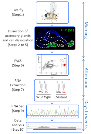
Figure 1: Overview of the protocol. Key steps of the protocol are shown, with the timeline on the right side. This procedure allows one starting with live Drosophila in the morning to have dissociated accessory gland cells by noon, sort them based on GFP expression, and get their RNAs extracted by the end of the working day. RNA sequencing and data analysis will typically take a few weeks. This figure has been modified from reference²⁷. Please click here to view a larger version of this figure.

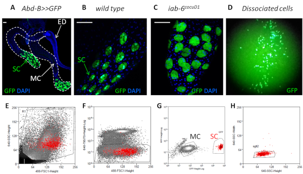
Figure 2: Isolating and sorting GFP-expressing secondary cells. (A) Confocal image of Abd-B:GAL4 UAS-GFP accessory gland expressing GFP in secondary cells (SC), but not in main cells (MC). Nuclei are stained with DAPI (blue). Dotted white line delimits AG lobes. ED is Ejaculatory duct. White bars in the upper left corner are 50 µm scales. (B,C) Enlarged views of accessory gland distal part with SC expressing GFP, in wild type (B) and iab-6^cocuD1 (C) background. (D) Dissociated cells at low magnification under the GFP binocular. (E-H) FACS gating strategy to purify SC and MC. Red dots on all panels shown SCs as defined in panel (G). First the debris are excluded (E, step 6.2.1) as well as the Draq-7 positive dead cells (F, step 6.2.2). GFP positive cells are selected (SC) as well as an homogeneous population of GFP negative cells (MC) (G, steps 6.2.4 and 6.2.5). Doublets are excluded from both MC and SC population (step 6.2.3, only the SSC-H vs SSC-W gating for SC is shown on 2H as an example). This figure has been modified from reference²⁷. Please click here to view a larger version of this figure.

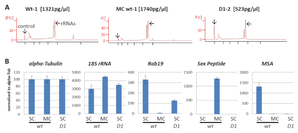
Figure 3: QC on RNAs: quality, quantity, and cell type specificity. (A) Control of RNA quality and concentration estimation on PicoChip. The 25 nt peak is the control for quantification. Low baseline indicates low degradation and the 2 major peaks are the ribosomal RNAs. The 3 samples used for RT-qPCR are shown, their quality is representative of all RNA samples used in this study, and their estimated concentrations reflect the variation in total RNA we obtained between samples. (B) RT-qPCR demonstrate the specificity of the sorting of secondary cells (SC) and main cells (MC). Gene expression quantification is done using the q=2^(40-Cq) formula. Each triplicate of each gene in each condition is normalized to the mean quantity of alpha-Tubulin RNA to compensate for total RNA variation. Error bars show standard deviation. WT means wild type and D1 refers to the iab-6^cocuD1 mutant. This figure has been modified from reference²⁷. Please click here to view a larger version of this figure.

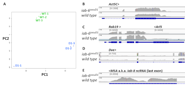
Figure 4: QC on RNA sequencing data. (A) Principal Components Analysis (PCA) on WT-1,-2,-3 (green dots) and D1-1,-2,-3 (blue dots) RNA sequencing datasets. (B-E) Sequencing reads mapped to the Drosophila reference genome using the IGV software. Only one representative sample of each genotype is shown for clarity sake (WT-1 and D1-2), and only a few specific loci are shown. Gene names are written on top of each panel, > and < symbols refer to their orientation. Numbers in brackets represent for each track the scale for the number of reads per DNA base pair. This scale is the same for both conditions for a given gene, but varies between genes for better visualization. Blue bars at the bottom of each panel show genes' introns (thin line), exons (wide line) and ORF (rectangles with >>). Note that Rab19 and Arl5 are overlapping, convergent genes (C). This figure has been modified from reference²⁷. Please click here to view a larger version of this figure.

Primers used for RT-qPCR in this study:
Target gene	Forward primer	Reverse primer
alpha-Tubulin	TTTTCCTTGTCGCGTGTGAA	CCAGCCTGACCAACATGGAT
18S rRNA	CTGAGAAACGGCTACCACATC	ACCAGACTTGCCCTCCAAT
Rab19	CAGGAGAGGTTTCGCACTATTAC	TTGGAAAAGGAAGACCGCTTG
Sex Peptide	GGAATGGCCGTGGAATAGGA	TAACATCTTCCACCCCAGGC
MSA	CTCATCTGCGTCTTCGCGTG	CAGCTCCGTTTGTAATCTCTCGAGC

Table 1: Primers sequence

Discussion

Methods for cell dissociation from Drosophila tissue like imaginal discs are already described²³. Our attempts to simply use these procedures on accessory glands failed, encouraging us to develop this new protocol. Protease digestion and mechanical trituration were critical steps we troubleshot for the success of the procedure, and we thus placed many notes in sections 2 to 5 to help experimenters to obtain satisfactory results. For dissociation to be successful, peptidases must reach the accessory gland cells, which are protected by the viscous seminal fluid in the lumen and the muscle layer around the gland. Dissecting the glands' distal part was thus critical (step 3.6). Also, digesting for 60 min at least with vigorous shaking (step 4.1) was necessary. Gentle dissociation with trypsin solution (e.g., TrypLE) preserved the gland integrity and cell viability until mechanical dissociation. The addition of either papain or collagenase in association with trypsin solution improved the dissociation (perfect dissociation was obtained with fewer pipetting, resulting in better cell survival). However, none of those enzymes were sufficient to dissociate the cells on their own. Pipetting using rounded narrow tips generated in part 2.2.2 is a key step for this method. Hence, this trituration (steps 5.2-5.3) should be optimized in small scale experiments to choose the best combination of tips (see note in step 5.3).

Using this protocol, one will be able to isolate 500 to 800 live secondary cells from 40 males. This represents ~20% (± 5%) recovery considering 3,200 SC as the starting material (40 males x 80 SC). 20% efficiency was high enough for RNA sequencing since we could process multiple samples in a day. However, this might be improved by several methods including: working in larger batches; doing trituration in the digestion tube and skipping step 5.4 to reduce transfers; triturating very gently (some dissociated GFP+ cells die shortly after step 5.3); shortening the period between dissociation and FACS; decreasing the digestion time by using trypsin solution at higher concentration; using less stringent parameters for singlet selection (step 6.2.3) and aborted sorting. One limitation of this protocol is that it takes several hours to isolate cells; hence it is not suited to study very transient gene expression changes. With this protocol, 4 x 20 males can be processed by a single person (with training) in one morning, allowing RNA extraction from SC of two different conditions in 1 day (Figure 1). Notably, more experimenters can participate in accessory glands collection (steps 3.1-3.3) in order to process multiple samples on the same day. However, steps 3.4 onwards will preferentially be performed by the same person to maximize reproducibility.

Secondary cells carry out essential functions for male fecundity^12,20,24, but the complete picture of the genes they express to fulfill this role is still missing. Here, we describe how to obtain the transcriptome of these cells from a relatively small number of flies, enabling the comparison of gene expression in SC in different conditions. Here, one mutant affecting SC function and morphology was used, and important changes in its transcriptome are visible. This method might thus help identifying new SC genes necessary for their function. To our knowledge, the only alternative method to obtain SC transcriptome was performed in our lab by manual picking of SCs. Good quality RNA sequencing data was obtained, but the procedure was too labor intensive to be performed in multiple conditions. We will compare our SC RNAseq datasets and analyze their biological meaning about SC biology in a distinct paper (in preparation).

In the future, this technique will not only shed light on wild type SC transcriptome, but also enable to study the impact of environment or gene alteration on accessory gland cells transcriptome. SC number, morphology and vacuolar content have been shown to depend on male diet, mating status and age^21,25,26. We still have a limited understanding of the genetic pathways involved and comparing SC transcriptomes in different conditions would be insightful. This fast and relatively simple protocol will enable such studies. Importantly, this method allows isolating main cells from the same individuals, and could thus be used as it is to determine whether genetic and environmental parameters affect both accessory gland cell types simultaneously.

Materials

List of materials used in this article

Name	Company	Catalog Number	Comments
24-wells Tissue Culture plate	VWR	734-2325
Binocular microscope for dissection
Binocular with light source for GFP
Bunsen
Draq7 0.3 mM	BioStatus	DR71000
Plastic microtubes 1.5 mL	Eppendorf
FACS	Beckman Coulter	MoFlo Astrios
Fine dissection forceps
Foetal bovine serum	Gibco	10270-106	heat inactivated prior to use
Glass dishes for dissection
Ice bucket
ImProm-II Reverse Transcription System	Promega	A3800
MasterPure RNA Purification Kit	Epicentre	MCR85102
Nextera XT kit	illumina		https://emea.illumina.com/products/by-type/sequencing-kits/library-prep-kits/nextera-xt-dna.html
P1000	Gilson
P20	Gilson
P200	Gilson
Papain			50U/mL stock
PBS			home made
Penicillin-Streptomycin	Gibco	15070-063
PolydT primers
Random hexamer primers
RNA 6000 Pico kit	Agilent
Schneider’s Drosophila medium	Gibco	21720-001
SMARTer cDNA synthesis kit	Takara		https://www.takarabio.com/products/cdna-synthesis/cdna-synthesis-kits/smarter-cdna-synthesis-kits
SYBR select Master mix for CFX	applied biosystems	4472942
Thermo Shaker	Hangzhou Allsheng intruments	MS-100
Tipone 1250 μL graduated tip	Starlab	S1161-1820
Tipone 200 μL bevelled tip	Starlab	S1161-1800
TrypLE Express Enzyme	Gibco	12604013
Vortex

References

- Avila, F. W., Sirot, L. K., LaFlamme, B. A., Rubinstein, C. D., Wolfner, M. F. Insect seminal fluid proteins: identification and function. Annual Review of Entomology. 56, 21-40 (2011).
- Carmel, I., Tram, U., Heifetz, Y. Mating induces developmental changes in the insect female reproductive tract. Current Opinion in Insect Science. 13, 106-113 (2016).
- League, G. P., Baxter, L. L., Wolfner, M. F., Harrington, L. C. Male accessory gland molecules inhibit harmonic convergence in the mosquito Aedes aegypti. Current Biology. 29 (6), R196-R197 (2019).
- Degner, E. C., et al. Proteins, Transcripts, and Genetic Architecture of Seminal Fluid and Sperm in the Mosquito Aedes aegypti. Molecular & Cellular Proteomics. 18 (Suppl 1), S6-S22 (2019).
- Wedell, N. Female receptivity in butterflies and moths. Journal of Experimental Biology. 208 (Pt 18), 3433-3440 (2005).
- Laflamme, B. A., Wolfner, M. F. Identification and function of proteolysis regulators in seminal fluid. Molecular Reproduction and Development. 80 (2), 80-101 (2013).
- Wilson, C., Leiblich, A., Goberdhan, D. C., Hamdy, F. The Drosophila Accessory Gland as a Model for Prostate Cancer and Other Pathologies. Current Topics in Developmental Biology. 121, 339-375 (2017).
- Kubli, E., Bopp, D. Sexual behavior: how Sex Peptide flips the postmating switch of female flies. Current Biology. 22 (13), R520-R522 (2012).
- Kubli, E. Sex-peptides: seminal peptides of the Drosophila male. Cellular and Molecular Life Sciences. 60 (8), 1689-1704 (2003).
- Liu, H., Kubli, E. Sex-peptide is the molecular basis of the sperm effect in Drosophila melanogaster. Proceedings of the National Academy of Sciences of the United States of America. 100 (17), 9929-9933 (2003).
- Ram, K. R., Wolfner, M. F. Sustained post-mating response in Drosophila melanogaster requires multiple seminal fluid proteins. PLoS Genetics. 3 (12), e238(2007).
- Sitnik, J. L., Gligorov, D., Maeda, R. K., Karch, F., Wolfner, M. F. The Female Post-Mating Response Requires Genes Expressed in the Secondary Cells of the Male Accessory Gland in Drosophila melanogaster. Genetics. 202 (3), 1029-1041 (2016).
- Avila, F. W., Wolfner, M. F. Acp36DE is required for uterine conformational changes in mated Drosophila females. Proceedings of the National Academy of Sciences of the United States of America. 106 (37), 15796-15800 (2009).
- Adams, E. M., Wolfner, M. F. Seminal proteins but not sperm induce morphological changes in the Drosophila melanogaster female reproductive tract during sperm storage. Journal of Insect Physiology. 53 (4), 319-331 (2007).
- Singh, A., et al. Long-term interaction between Drosophila sperm and sex peptide is mediated by other seminal proteins that bind only transiently to sperm. Insect Biochemistry and Molecular Biology. 102, 43-51 (2018).
- Avila, F. W., Wolfner, M. F. Cleavage of the Drosophila seminal protein Acp36DE in mated females enhances its sperm storage activity. Journal of Insect Physiology. 101, 66-72 (2017).
- Chapman, T., Davies, S. J. Functions and analysis of the seminal fluid proteins of male Drosophila melanogaster fruit flies. Peptides. 25 (9), 1477-1490 (2004).
- Gligorov, D., Sitnik, J. L., Maeda, R. K., Wolfner, M. F., Karch, F. A novel function for the Hox gene Abd-B in the male accessory gland regulates the long-term female post-mating response in Drosophila. PLoS Genetics. 9 (3), e1003395(2013).
- Minami, R., et al. The homeodomain protein defective proventriculus is essential for male accessory gland development to enhance fecundity in Drosophila. PLoS One. 7 (3), e32302(2012).
- Maeda, R. K., et al. The lncRNA male-specific abdominal plays a critical role in Drosophila accessory gland development and male fertility. PLoS Genetics. 14 (7), e1007519(2018).
- Prince, E., et al. Rab-mediated trafficking in the secondary cells of Drosophila male accessory glands and its role in fecundity. Traffic. 20 (2), 137-151 (2019).
- Robinson, M. D., Oshlack, A. A scaling normalization method for differential expression analysis of RNA-seq data. Genome Biology. 11 (3), R25(2010).
- Khan, S. J., Abidi, S. N., Tian, Y., Skinner, A., Smith-Bolton, R. K. A rapid, gentle and scalable method for dissociation and fluorescent sorting of imaginal disc cells for mRNA sequencing. Fly (Austin). 10 (2), 73-80 (2016).
- Corrigan, L., et al. BMP-regulated exosomes from Drosophila male reproductive glands reprogram female behavior. Journal of Cell Biology. 206 (5), 671-688 (2014).
- Leiblich, A., et al. Bone morphogenetic protein- and mating-dependent secretory cell growth and migration in the Drosophila accessory gland. Proceedings of the National Academy of Sciences of the United States of America. 109 (47), 19292-19297 (2012).
- Kubo, A., et al. Nutrient conditions sensed by the reproductive organ during development optimize male fecundity in Drosophila. Genes to Cells. 23 (7), 557-567 (2018).
- Immarigeon, C., Karch, F., Maeda, R. K. FACS-based isolation and RNA extraction of Secondary Cells from the Drosophila male Accessory Gland. bioRxiv. , 630335(2019).
Reprints and Permissions